Grouping Data Methods of cluster analysis Goals 1

Grouping Data Methods of cluster analysis

Goals 1 1. We want to identify groups of similar artifacts or features or sites or graves, etc that represent cultural, functional, or chronological differences 2. We want to create groups as a measurement technique to see how they vary with external variables

Goals 2 3. We want to cluster artifacts or sites based on their location to identify spatial clusters

Real vs. Created Types • Differences in goals – Real types are the aim of Goal 1 – Created types are the aim of Goal 2 • Debate over whether Real types can be discovered with any degree of certainty • Cluster analysis guarantees groups – you must confirm their utility

Initial Decisions 1 • What variables to use? – All possible – Constructed variables (from principal components, correspondence analysis, or multi-dimensional scaling) – Restricted set of variables that support the goal(s) of creating groups (e. g. functional groups, cultural or stylistic groups)

Initial Decisions 2 • How to transform the variables? – Log transforms – Conversion to percentages (to weight rows equally) – Size standardization (dividing by geometric mean) – Z – scores (to weight columns equally) – Conversion of categorical variables

Initial Decisions 3 • How to measure distance? – Types of variables – Goals of the analysis – If uncertain, try multiple methods

Methods of Grouping • Partitioning Methods – divide the data into groups • Hierarchical Methods – Agglomerating – from n clusters to 1 cluster – Divisive – from 1 cluster to k clusters

Partitioning • K – Means, K – Medoids, Fuzzy • Measure of distance – but do not need to compute full distance matrix • Specify number of groups in advance • Minimizing within group variability • Finds spherical clusters

Procedure • Start with centers for k groups (usersupplied or random) • Repeat up to iter. max times (default 10) – Allocate rows to their closest center – Recalculate the center positions • Stop • Different criteria for allocation • Use multiple starts (e. g. 5 – 15)

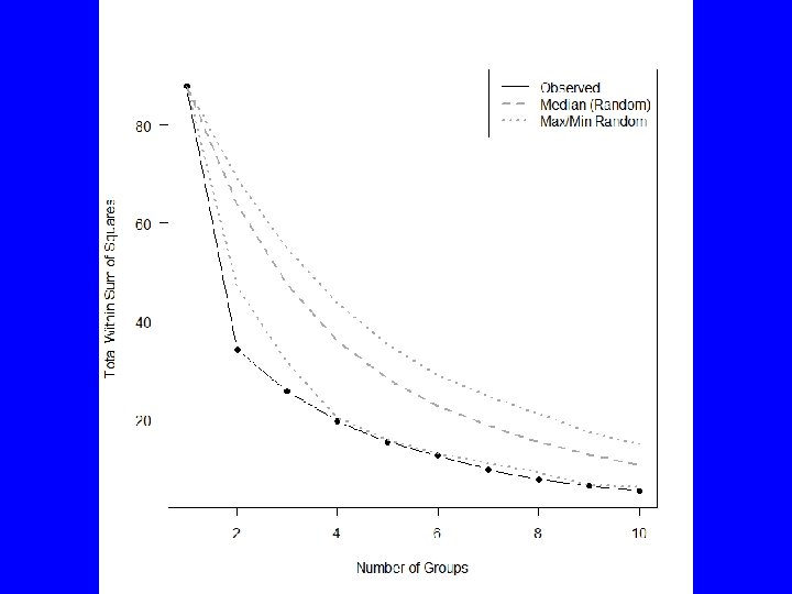
Evaluation 1 • Compute groups for a range of cluster sizes and plot within group sums of squares to look for sharp increases • Cluster randomized versions of the data and compare the results • Examine table of statistics by group

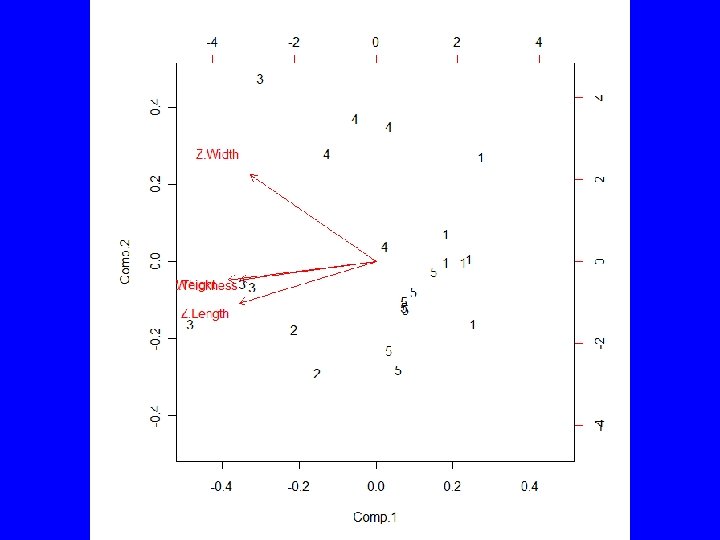
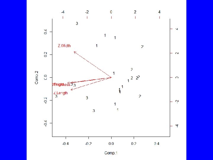
Evaluation 2 • Plot groups in two dimensions with PCA, or MDS • Compare the groups using data or information not included in the analysis

Partitioning Using R • Base R includes kmeans() forming groups by partitioning • Rcmdr includes KMeans() to iterate kmeans() for best solution • Package cluster() includes pam() which uses medoids for more robust grouping and fanny() which forms fuzzy clusters

Example • Darl. Points (not Dart. Points) has 4 measurements for 23 Darl points • Create Z-scores to weight variables equally with Data | Manage variables in active data set | Standardize variables … • (or could use PCA and PC Scores)

Example (cont) • Use Rcmdr to partition the data into 5, 4, 3, and 2 groups • Statistics | Dimensional analysis | Cluster analysis | k-means cluster analysis … • TWSS = 15. 42, 19. 78, 25. 83, 34. 24 • Select group number and have Rcmdr add group to data set

Evaluation • Evaluate groups against randomized data – Randomly permute each variable – Run k-means – Compare random and non-random results • Evaluate groups against external criteria (location, material, age, etc)

KMPlot. WSS <- function(data, ming, maxg) { WSS <- sapply(ming: maxg, function(x) kmeans(data, centers = x, iter. max = 10, nstart = 10)$tot. withinss) plot(ming: maxg, WSS, las=1, type="b", xlab="Number of Groups", ylab="Total Within Sum of Squares", pch=16) print(WSS) } KMRand. WSS <- function(data, samples, min, max) { KRand <- function(data, min, max){ Rnd <- apply(data, 2, sample) sapply(min: max, function(y) kmeans(Rnd, y, iter. max= 10, nstart=5)$tot. withinss) } Sim <- sapply(1: samples, function(x) KRand(data, min, max)) t(apply(Sim, 1, quantile, c(0, . 005, . 01, . 025, . 975, . 995, 1))) }

# Compare data to randomized sets KMPlot. WSS(Darl. Points[, 6: 9], 1, 10) Qtiles <- KMRand. WSS(Darl. Points[, 6: 9], 2000, 1, 10) matlines(1: 10, Qtiles[, c(1, 5, 9)], lty=c(3, 2, 3), lwd=2, col="dark gray") legend("topright", c("Observed", "Median (Random)", "Max/Min Random"), col=c("black", "dark gray"), lwd=c(1, 2, 2), lty=c(1, 2, 3))

Hierarchical Methods • Agglomerative – successive merging • Divisive - successive splitting – Monothetic – binary data – Polythetic – interval/ratio

Agglomerative • At the start all rows are in separate groups (n groups or clusters) • At each stage two rows are merged, a row and a group are merged, or two groups are merged • The process stops when all rows are in a single cluster

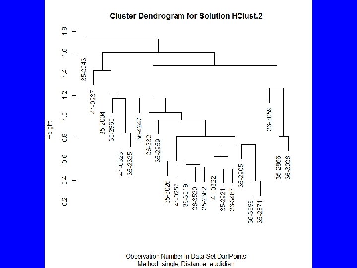
Agglomeration Methods • How should clusters be formed? – Single Linkage, irregular shape groups – Average Linkage – spherical groups – Complete Linkage – spherical groups – Ward’s Method – spherical groups – Median – dendrogram inversions – Centroid – dendrogram inversions – Mc. Quitty – similarity by reciprocal pairs

Agglomerating with R • Base R includes hclus() forming groups by partitioning • Package cluster() includes agnes() • Rcmdr uses hclus() via Statistics | Dimensional analysis | Cluster analysis | Hierarchical cluster analysis …

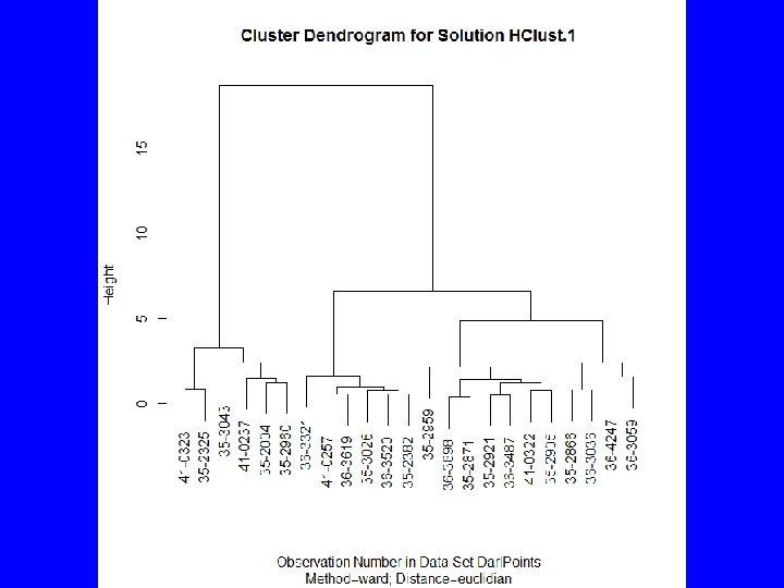
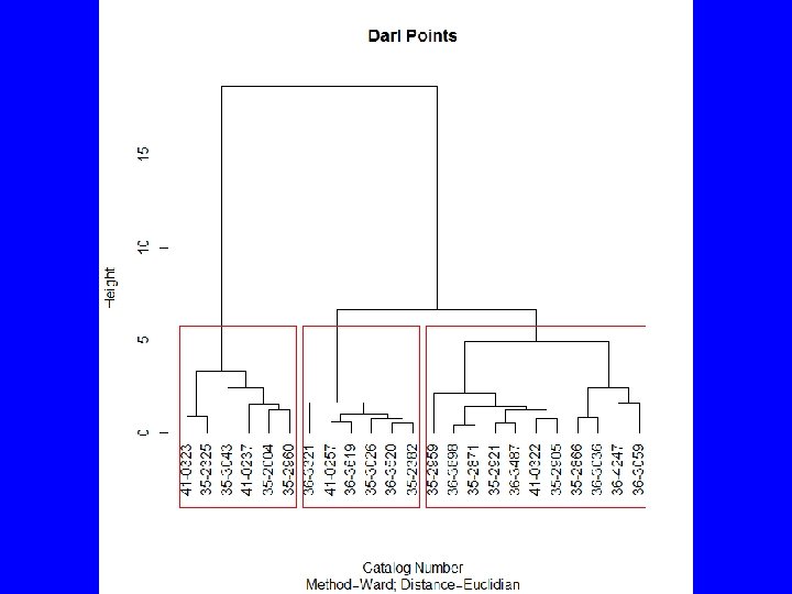
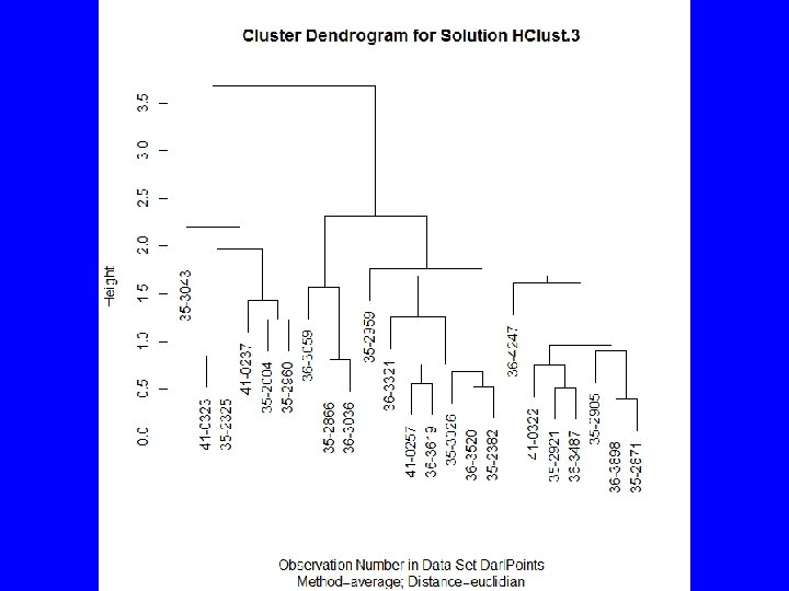
HClust • Rcmdr menus provide – Cluster analysis and plot – Summary statistics by group – Adding cluster to data set • To get traditional dendrogram: – plot(HClust. 1, hang=-1, main= "Darl Points", xlab= "Catalog Number", sub="Method=Ward; Distance=Euclidian") – rect. hclust(HClust. 1, 3)

summary(as. factor(cutree(HClust. 1, k = 3))) # Cluster Sizes 1 2 3 11 6 6 by(model. matrix(~-1 + Z. Length + Z. Thickness + Z. Weight + Z. Width, Darl. Points), as. factor(cutree(HClust. 1, k = 3)), mean) # Cluster Centroids INDICES: 1 Z. Length Z. Thickness Z. Weight Z. Width -0. 1345150 -0. 1585615 -0. 2523805 -0. 1241642 ------------------------------INDICES: 2 Z. Length Z. Thickness Z. Weight Z. Width -1. 1085541 -0. 9209550 -0. 9400026 -0. 8200594 ------------------------------INDICES: 3 Z. Length Z. Thickness Z. Weight Z. Width 1. 355165 1. 211651 1. 402700 1. 047694 > biplot(princomp(model. matrix(~-1 + Z. Length + Z. Thickness + Z. Weight + Z. Width, Darl. Points)), xlabs = as. character(cutree(HClust. 1, k = 3)))

> cbind(HClust. 1$merge, HClust. 1$height) [, 1] [, 2] [, 3] [1, ] -12 -13 0. 3983821 [2, ] -2 -3 0. 5112670 [3, ] -9 -14 0. 5247650 [4, ] -10 -17 0. 5572146 [5, ] -15 3 0. 7362171 [6, ] -1 -11 0. 7471874 [7, ] -6 -18 0. 8120594 [8, ] -7 -8 0. 8491895 [9, ] 4 5 0. 9841552 [10, ] 2 6 1. 2150606 [11, ] -19 -21 1. 2300507 [12, ] 1 10 1. 4059158 [13, ] -22 11 1. 4963400 [14, ] -16 -20 1. 5800167 [15, ] -4 9 1. 6195709 [16, ] -5 12 2. 1556543 [17, ] -23 13 2. 4007863 [18, ] 7 14 2. 4252670 [19, ] 8 17 3. 2632812 [20, ] 16 18 4. 9021149 [21, ] 15 20 6. 6290417 [22, ] 19 21 18. 7730146

Divisive • At the start all rows are considered to be a single group • At each stage a group is divided into two groups based on the average dissimilarities • The process stops when all rows are in separate clusters