General Procedure for Finite Element Method FEM is


 6. Nodes to provide prescribed boundary condition.")


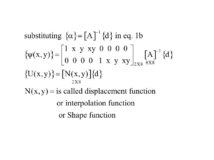
 (1 b)")
 This results in as many conditions as the number of unknown constants.")
 in eq. 1 a, following matrix")


- Slides: 18
General Procedure for Finite Element Method FEM is based on Direct Stiffness approach or Displacement approach. A broad procedural outline is listed below 1. Discretize and select element type. Skeletal structures Skeletal structure gets discretized naturally. Member between two joints are treated as an element. Continuums Arbitrary discretization.
Precautions to be taken while discretization. 1. Provide nodes wherever geometry changes 2. Provide a set of nodes along bimaterial interface, so that no single element encompass or cover both materials. Element should cover one material. 3. Nodes at such points where concentrated load acts. 4. Nodes at points of specific interest for the analyst. 5. Nodes/|elements are provided such that distributed loads are covered completely by the element edge. Distributed load shall not be applied partially on any element edge.
Precautions to be taken while discretization (contd) 6. Nodes to provide prescribed boundary condition. 7. Fine mesh in the regions of steep stress gradient. 8. Use symmetry condition 9 Aspect ratio of element 1 10. Avoid obtuse/acute angle 11. Node numbering along shorter direction.
Fundamental concept of FEM Consider a bar subjected to some exicitations like heating at one end. Let the field quantity flow through the body as fig 2, which has been obtained by solving governing DE/PDE, In FEM the domain is subdivided into subdomain and in each subdomain a piecewise continuous function is assumed. The fundamental concept of FEM is that continuous function of a continuum (given domain ) having infinite degrees of freedom is replaced by a discrete model, approximated by a set of piecewise continuous function having a finite degree of freedom. Thus the method got the name finite element coined by Clough(1960). Fig. 2
2. Select displacement function e In the displacement approach a displacement function is assumed for uj ui the element. For example i For a one dimensional element j ui uj u(x) = a 1 + a 2 x uk i u(x) = a 1 + a 2 x + a 3 x 2 k j
For two dimensional rectangular elements displacement field at any interior of element is given by u(x, y) = a 1 + a 2 x + a 3 y + a 4 xy v(x, y) = a 5 + a 6 x + a 7 y + a 8 xy Pascal triangle for 2 D problems The terms for displacement function is selected symmetrically from the pascal triangle to maintain geometric isotropy
Pascal triangle for 3 D problems
(1 a) (1 b)
(2) This results in as many conditions as the number of unknown constants.
Using nodal boundary condition listed in eq. (2) in eq. 1 a, following matrix eqn. Can be obtained For quadrilateral element [A] is of size 8 X 8
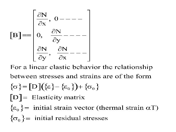
3. Establish strain displacement and stress/strain relationship. For one dimensional element For two dimensional element
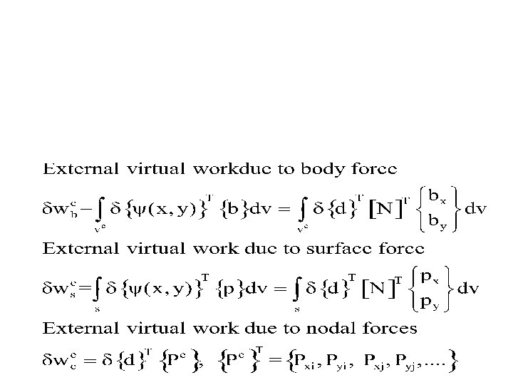
4. Establish equilibrium equation to develop element stiffness relation. Virtual work principle of a deformable body in equilibrium is subjected to arbitrary virtual displacement satisfying compatibility condition (admissible displacement), then the virtual work done by external(loads will be equal to virtual strain energy of internal stresses.
For equilibrium internal virtual work = external virtual work
First term in {fe} is equivalent nodal force vector due to initial strain. Second term is equivalent nodal force vector due to initial stress. Third term is equivalent nodal force vector due to body force. Fourth term is equivalent nodal force vector due to surface traction. Last term is applied concentrated load vector