Feature description and matching Matching feature points We

Feature description and matching

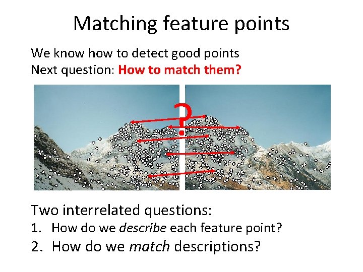
Matching feature points We know how to detect good points Next question: How to match them? ? Two interrelated questions: 1. How do we describe each feature point? 2. How do we match descriptions?

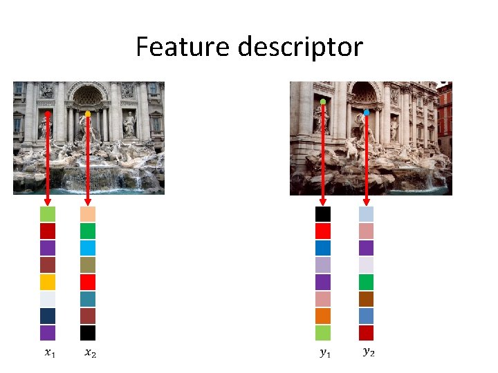
Feature descriptor

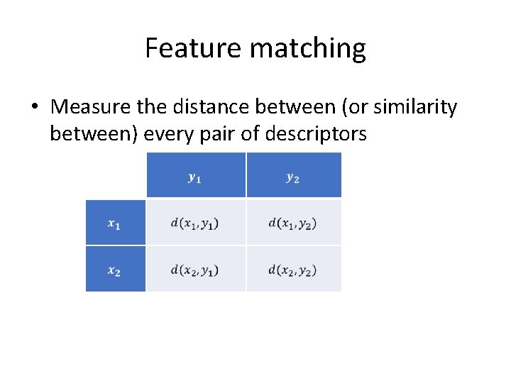
Feature matching • Measure the distance between (or similarity between) every pair of descriptors

Invariance vs. discriminability • Invariance: – Distance between descriptors should be small even if image is transformed • Discriminability: – Descriptor should be highly unique for each point (far away from other points in the image)

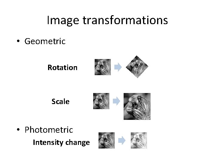
Image transformations • Geometric Rotation Scale • Photometric Intensity change

Invariance • Most feature descriptors are designed to be invariant to – Translation, 2 D rotation, scale • They can usually also handle – Limited 3 D rotations (SIFT works up to about 60 degrees) – Limited affine transformations (some are fully affine invariant) – Limited illumination/contrast changes

How to achieve invariance Design an invariant feature descriptor – Simplest descriptor: a single 0 • What’s this invariant to? • Is this discriminative? – Next simplest descriptor: a single pixel • What’s this invariant to? • Is this discriminative?

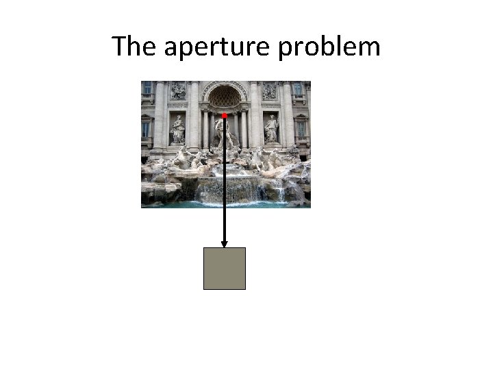
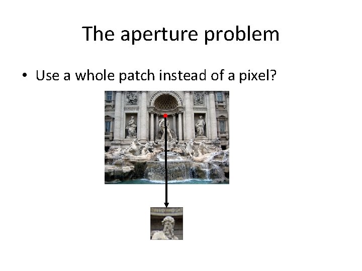
The aperture problem

The aperture problem • Use a whole patch instead of a pixel?

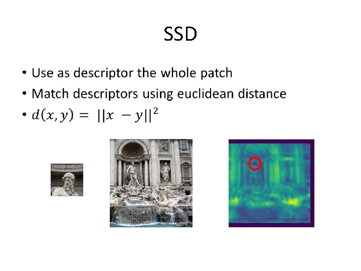
SSD •

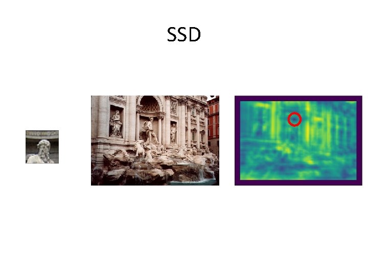
SSD

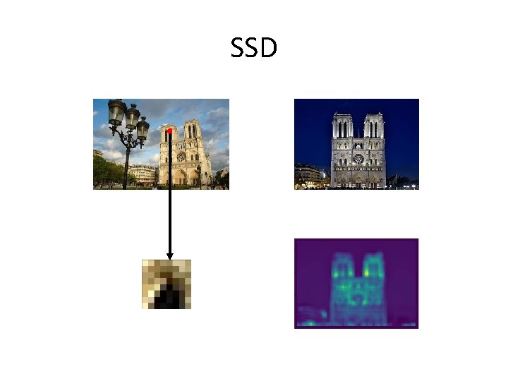
SSD

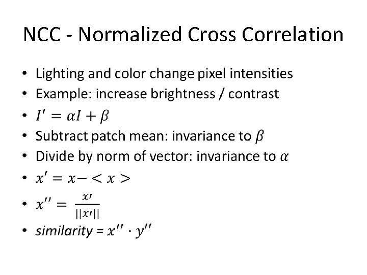
NCC - Normalized Cross Correlation •

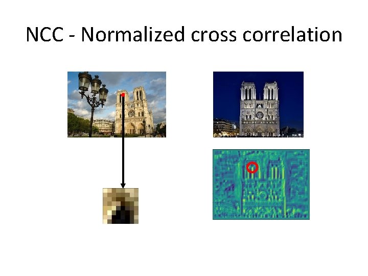
NCC - Normalized cross correlation

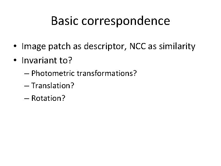
Basic correspondence • Image patch as descriptor, NCC as similarity • Invariant to? – Photometric transformations? – Translation? – Rotation?

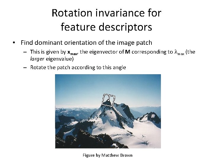
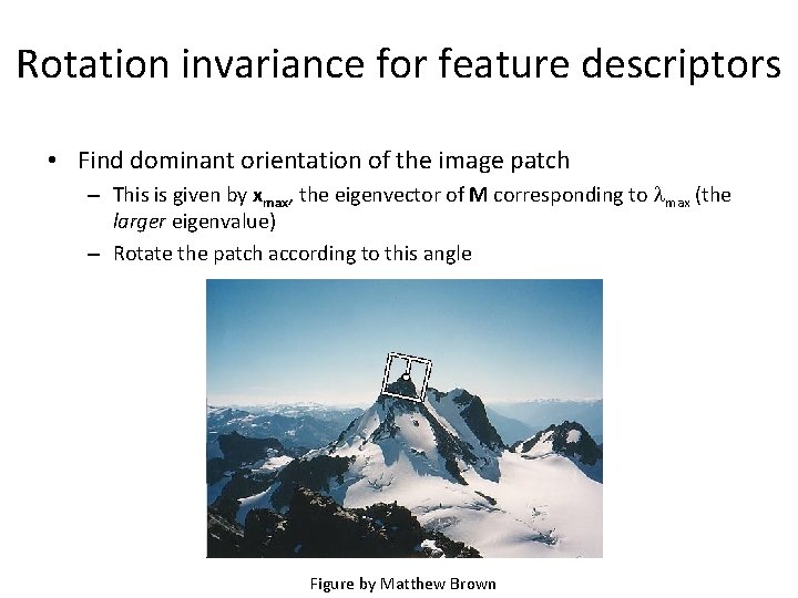
Rotation invariance for feature descriptors • Find dominant orientation of the image patch – This is given by xmax, the eigenvector of M corresponding to max (the larger eigenvalue) – Rotate the patch according to this angle Figure by Matthew Brown

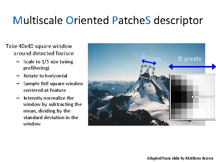
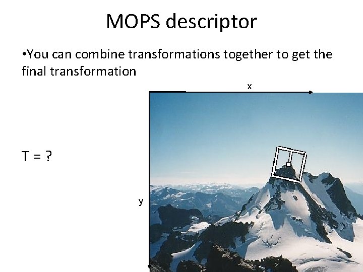
Multiscale Oriented Patche. S descriptor Take 40 x 40 square window around detected feature – Scale to 1/5 size (using prefiltering) – Rotate to horizontal – Sample 8 x 8 square window centered at feature – Intensity normalize the window by subtracting the mean, dividing by the standard deviation in the window 40 pi xels 8 pixels CSE 576: Computer Vision Adapted from slide by Matthew Brown

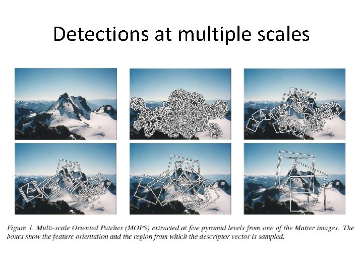
Detections at multiple scales

Rotation invariance for feature descriptors • Find dominant orientation of the image patch – This is given by xmax, the eigenvector of M corresponding to max (the larger eigenvalue) – Rotate the patch according to this angle Figure by Matthew Brown

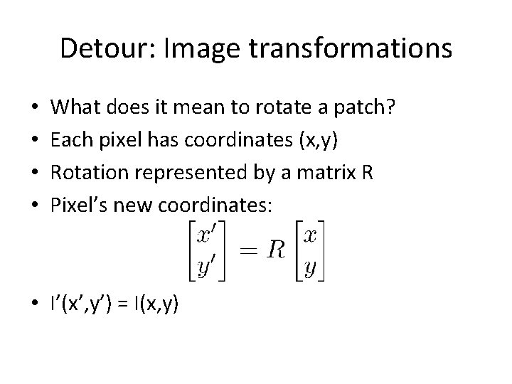
Detour: Image transformations • • What does it mean to rotate a patch? Each pixel has coordinates (x, y) Rotation represented by a matrix R Pixel’s new coordinates: • I’(x’, y’) = I(x, y)

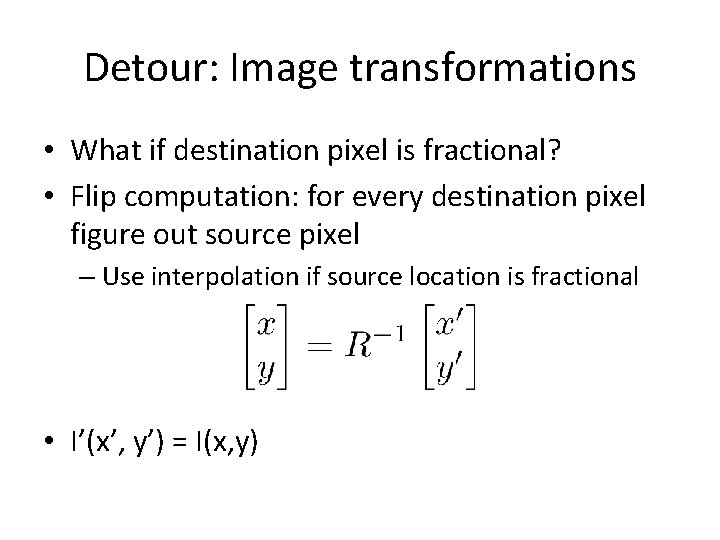
Detour: Image transformations • What if destination pixel is fractional? • Flip computation: for every destination pixel figure out source pixel – Use interpolation if source location is fractional • I’(x’, y’) = I(x, y)

Multiscale Oriented Patche. S descriptor Take 40 x 40 square window around detected feature – Scale to 1/5 size (using prefiltering) – Rotate to horizontal – Sample 8 x 8 square window centered at feature – Intensity normalize the window by subtracting the mean, dividing by the standard deviation in the window 40 pi xels 8 pixels CSE 576: Computer Vision Adapted from slide by Matthew Brown

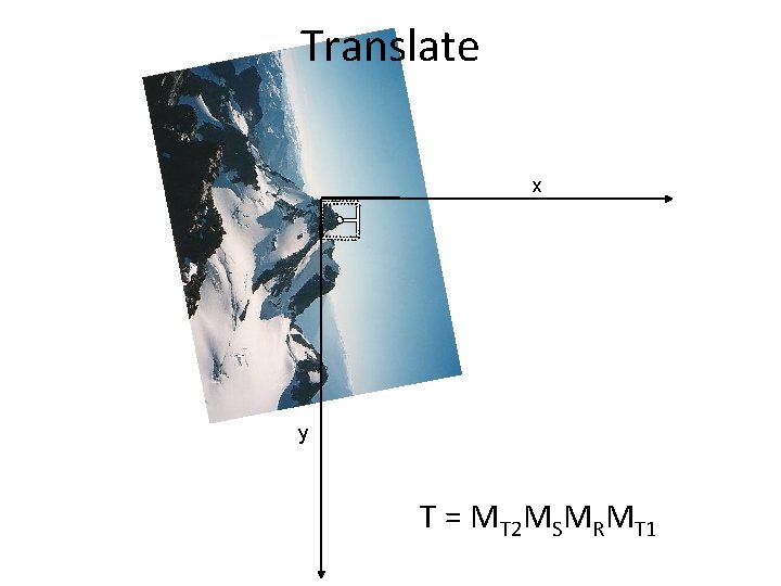
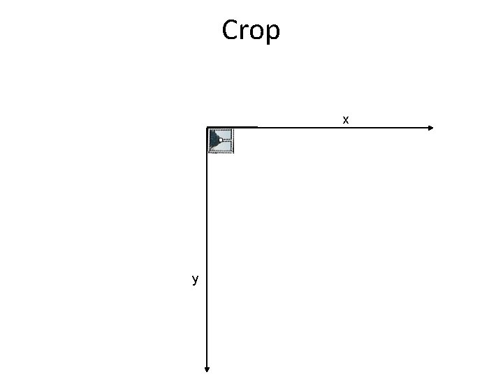
MOPS descriptor • You can combine transformations together to get the final transformation x T = ? y

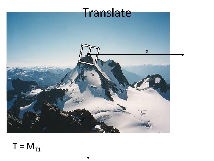
Translate x y T = MT 1

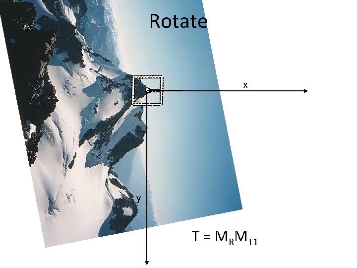
Rotate x y T = MRMT 1

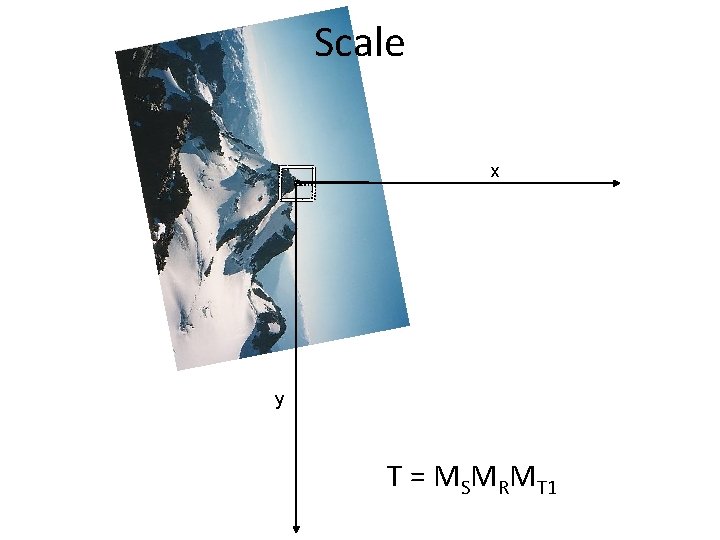
Scale x y T = MSMRMT 1

Translate x y T = MT 2 MSMRMT 1

Crop x y

Detections at multiple scales

Invariance of MOPS • Intensity • Scale • Rotation

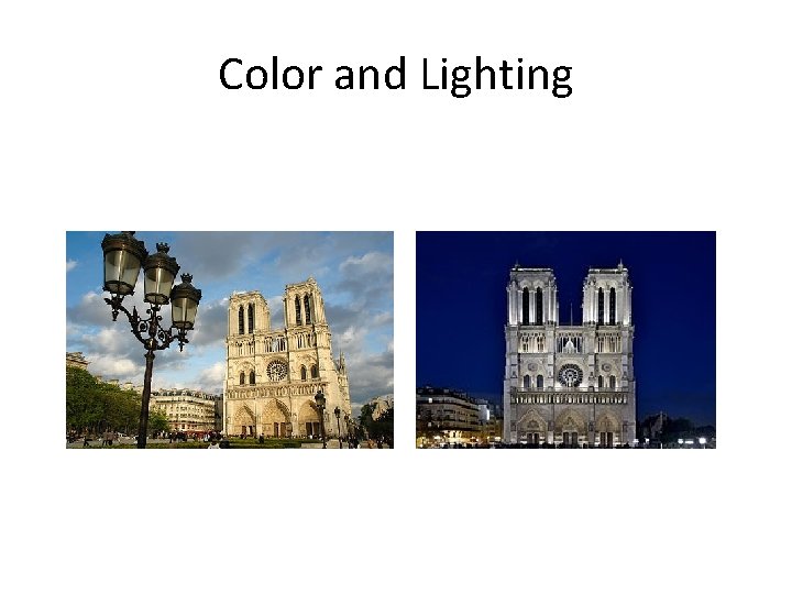
Color and Lighting

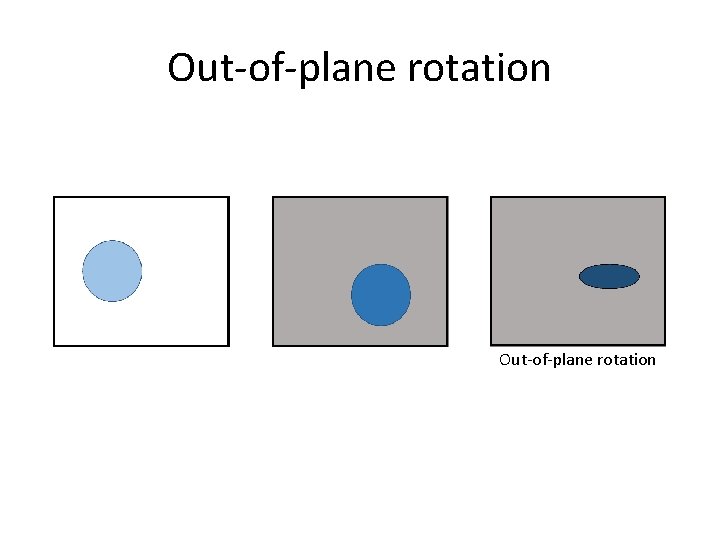
Out-of-plane rotation

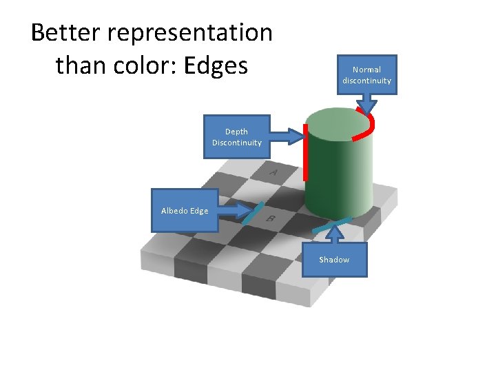
Better representation than color: Edges Normal discontinuity Depth Discontinuity Albedo Edge Shadow

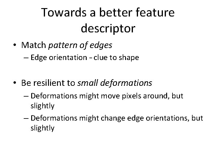
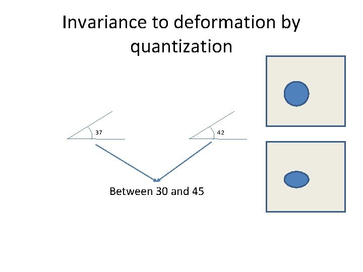
Towards a better feature descriptor • Match pattern of edges – Edge orientation – clue to shape • Be resilient to small deformations – Deformations might move pixels around, but slightly – Deformations might change edge orientations, but slightly

Invariance to deformation by quantization 37 42 Between 30 and 45

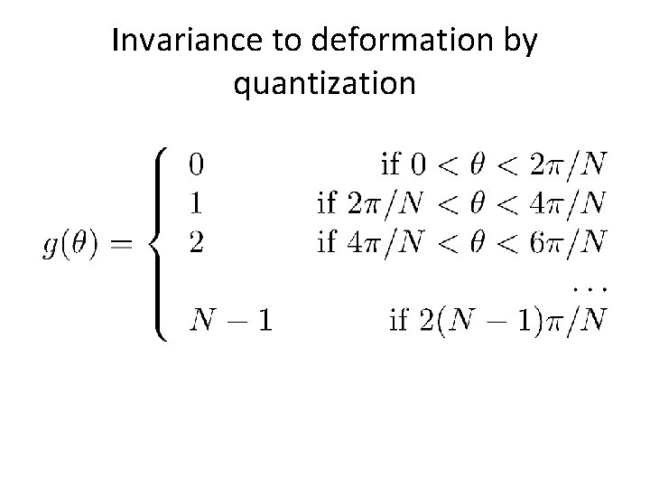
Invariance to deformation by quantization

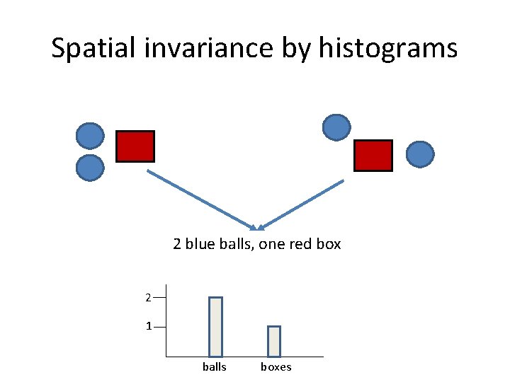
Spatial invariance by histograms 2 blue balls, one red box 2 1 balls boxes

Rotation Invariance by Orientation Normalization [Lowe, SIFT, 1999] • Compute orientation histogram • Select dominant orientation • Normalize: rotate to fixed orientation 0 T. Tuytelaars, B. Leibe 2

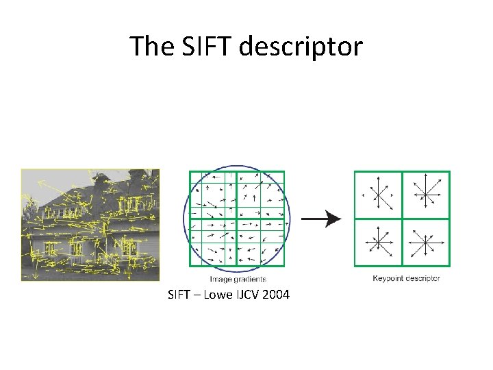
The SIFT descriptor SIFT – Lowe IJCV 2004

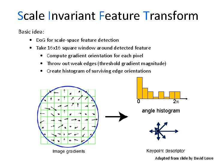
Scale Invariant Feature Transform Basic idea: • Do. G for scale-space feature detection • Take 16 x 16 square window around detected feature • Compute gradient orientation for each pixel • Throw out weak edges (threshold gradient magnitude) • Create histogram of surviving edge orientations 0 2 angle histogram Adapted from slide by David Lowe

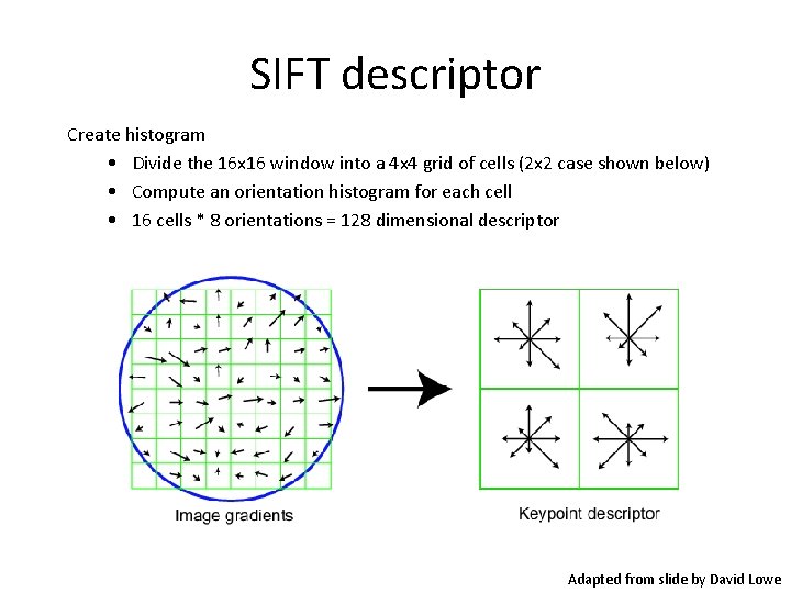
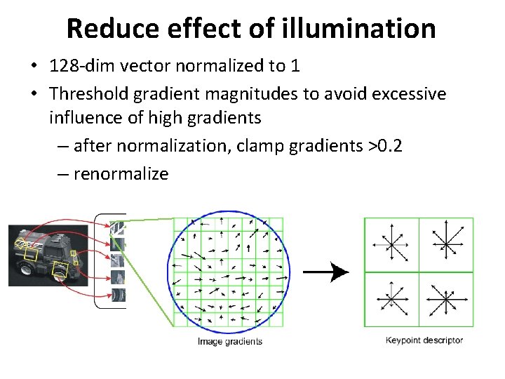
SIFT descriptor Create histogram • Divide the 16 x 16 window into a 4 x 4 grid of cells (2 x 2 case shown below) • Compute an orientation histogram for each cell • 16 cells * 8 orientations = 128 dimensional descriptor Adapted from slide by David Lowe

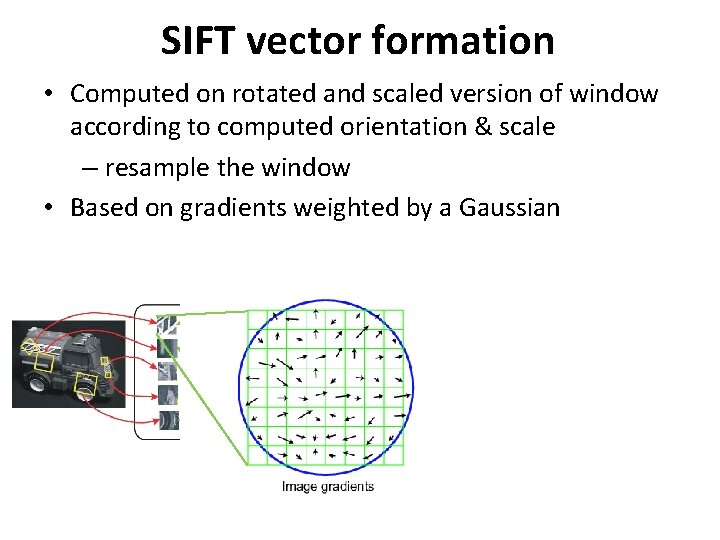
SIFT vector formation • Computed on rotated and scaled version of window according to computed orientation & scale – resample the window • Based on gradients weighted by a Gaussian

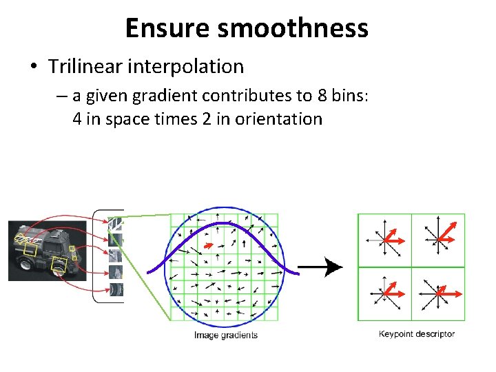
Ensure smoothness • Trilinear interpolation – a given gradient contributes to 8 bins: 4 in space times 2 in orientation

Reduce effect of illumination • 128 -dim vector normalized to 1 • Threshold gradient magnitudes to avoid excessive influence of high gradients – after normalization, clamp gradients >0. 2 – renormalize

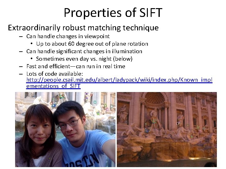
Properties of SIFT Extraordinarily robust matching technique – Can handle changes in viewpoint • Up to about 60 degree out of plane rotation – Can handle significant changes in illumination • Sometimes even day vs. night (below) – Fast and efficient—can run in real time – Lots of code available: http: //people. csail. mit. edu/albert/ladypack/wiki/index. php/Known_impl ementations_of_SIFT

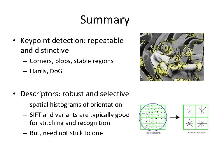
Summary • Keypoint detection: repeatable and distinctive – Corners, blobs, stable regions – Harris, Do. G • Descriptors: robust and selective – spatial histograms of orientation – SIFT and variants are typically good for stitching and recognition – But, need not stick to one

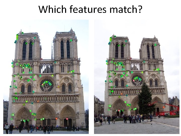
Which features match?

Feature matching Given a feature in I 1, how to find the best match in I 2? 1. Define distance function that compares two descriptors 2. Test all the features in I 2, find the one with min distance

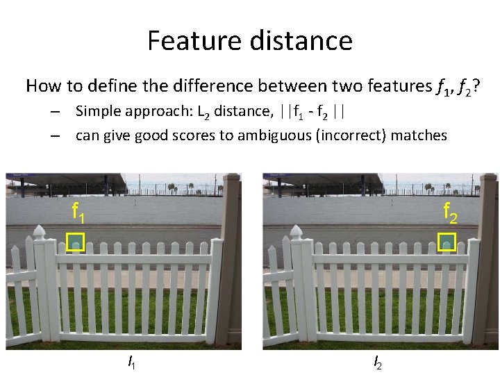
Feature distance How to define the difference between two features f 1, f 2? – Simple approach: L 2 distance, ||f 1 - f 2 || – can give good scores to ambiguous (incorrect) matches f 1 f 2 I 1 I 2

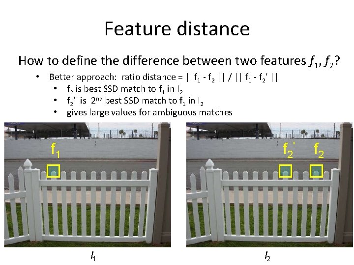
Feature distance How to define the difference between two features f 1, f 2? • Better approach: ratio distance = ||f 1 - f 2 || / || f 1 - f 2’ || • f 2 is best SSD match to f 1 in I 2 • f 2’ is 2 nd best SSD match to f 1 in I 2 • gives large values for ambiguous matches f 1 f 2' I 1 I 2 f 2