Exam 3 Review Zuyin Alvin Zheng Important Notes

Exam #3 Review Zuyin (Alvin) Zheng

Important Notes o Time 2 hours NOT 50 minutes ü Monday, May 8, 8: 00 am – 10: 00 am o Location ü Regular Class Room Alter Hall 231 o Calculator ü Do please bring your own calculator ü You will NOT be allowed to share calculators during the exam

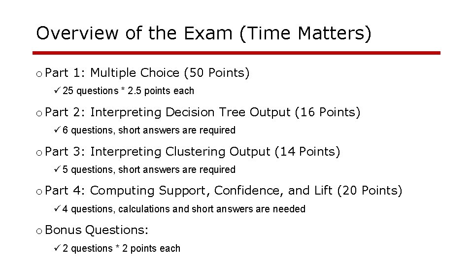
Overview of the Exam (Time Matters) o Part 1: Multiple Choice (50 Points) ü 25 questions * 2. 5 points each o Part 2: Interpreting Decision Tree Output (16 Points) ü 6 questions, short answers are required o Part 3: Interpreting Clustering Output (14 Points) ü 5 questions, short answers are required o Part 4: Computing Support, Confidence, and Lift (20 Points) ü 4 questions, calculations and short answers are needed o Bonus Questions: ü 2 questions * 2 points each

Using R and R-Studio

R and R-Studio o Open source, free o Many, many statistical add-on “packages” that perform data analysis o R Packages contain additional functionality (The base/engine) o Integrated Development Environment for R o Nicer interface that makes R easier to use o Requires R to run (The pretty face)

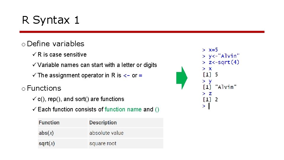
R Syntax 1 o Define variables ü R is case sensitive ü Variable names can start with a letter or digits ü The assignment operator in R is <- or = o Functions ü c(), rep(), and sort() are functions ü Each function consists of function name and ()

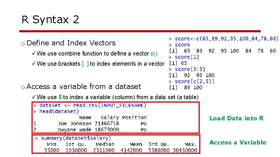
R Syntax 2 o Define and Index Vectors ü We use combine function to define a vector c() ü We use brackets [ ] to index elements in a vector o Access a variable from a dataset ü We use $ to index a variable (column) from a data set (a table) Load Data into R Access a Variable

Understanding Descriptive Statistics

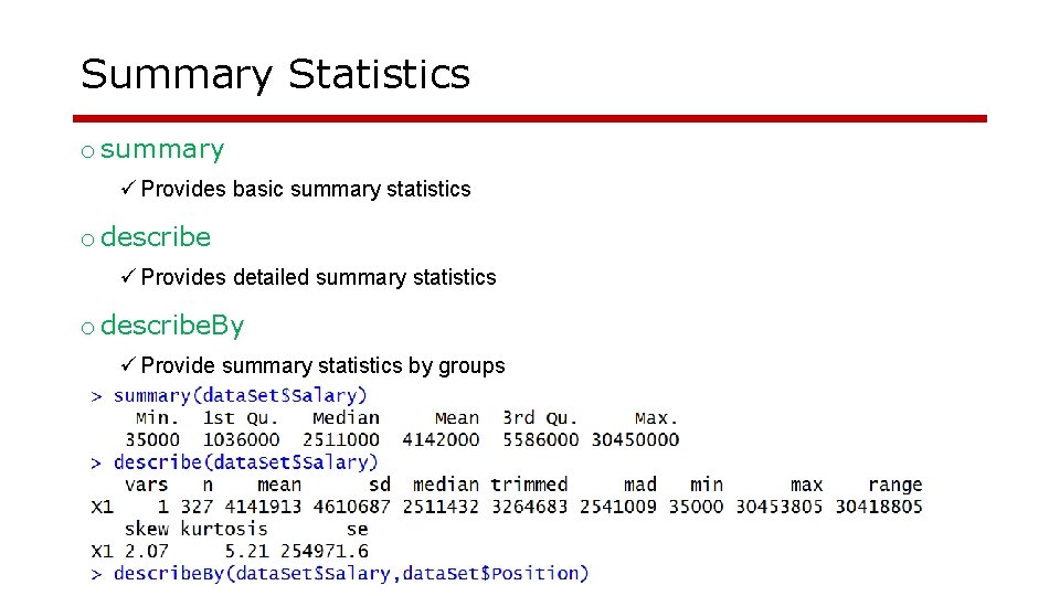
Summary Statistics o summary ü Provides basic summary statistics o describe ü Provides detailed summary statistics o describe. By ü Provide summary statistics by groups

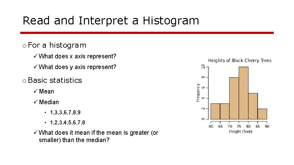
Read and Interpret a Histogram o For a histogram ü What does x axis represent? ü What does y axis represent? o Basic statistics ü Mean ü Median • 1, 3, 3, 6, 7, 8, 9 • 1, 2, 3, 4, 5, 6, 7, 8 ü What does it mean if the mean is greater (or smaller) than the median?

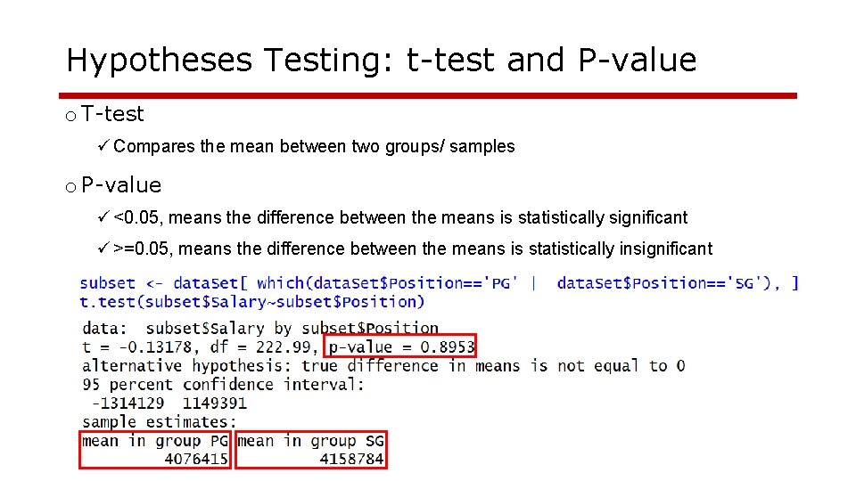
Hypotheses Testing: t-test and P-value o T-test ü Compares the mean between two groups/ samples o P-value ü <0. 05, means the difference between the means is statistically significant ü >=0. 05, means the difference between the means is statistically insignificant

Decision Tree Analysis

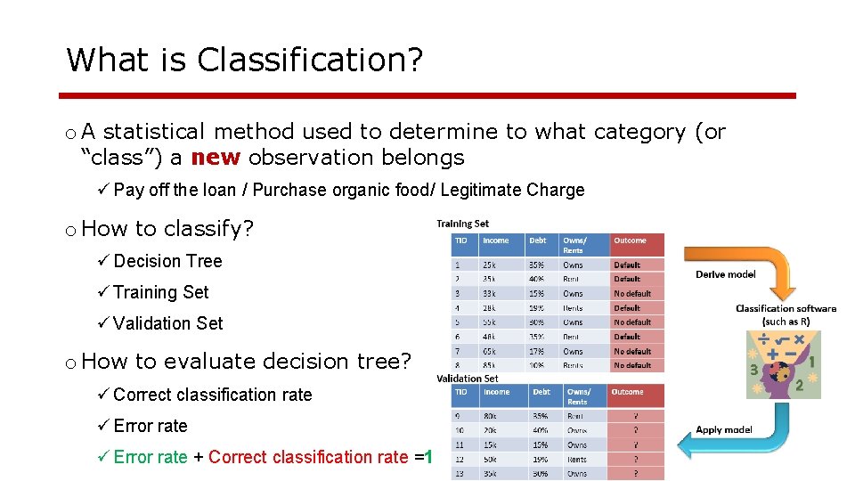
What is Classification? o A statistical method used to determine to what category (or “class”) a new observation belongs ü Pay off the loan / Purchase organic food/ Legitimate Charge o How to classify? ü Decision Tree ü Training Set ü Validation Set o How to evaluate decision tree? ü Correct classification rate ü Error rate + Correct classification rate =1

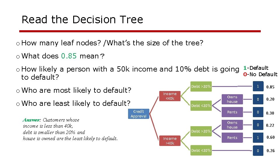
Read the Decision Tree o How many leaf nodes? /What’s the size of the tree? o What does 0. 85 mean？ o How likely a person with a 50 k income and 10% debt is going 1 -Default 0 -No Default to default? o Who are most likely to default? o Who are least likely to default? Answer: Customers whose income is less than 40 k, debt is smaller than 20% and house is owned are the least likely to default. 1 0. 85 Owns house 0 0. 20 Rents 0 0. 30 Owns house 0 0. 22 Rents 1 0. 60 0 0. 26 Debt >20% Income <40 k Debt <20% Credit Approval Debt >20% Income >40 k Debt <20%

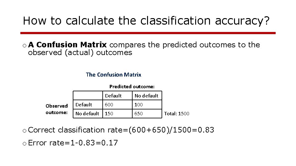
How to calculate the classification accuracy? o A Confusion Matrix compares the predicted outcomes to the observed (actual) outcomes The Confusion Matrix Predicted outcome: Observed outcome: Default No default Default 600 100 No default 150 650 Total: 1500 o Correct classification rate=(600+650)/1500=0. 83 o Error rate=1 -0. 83=0. 17

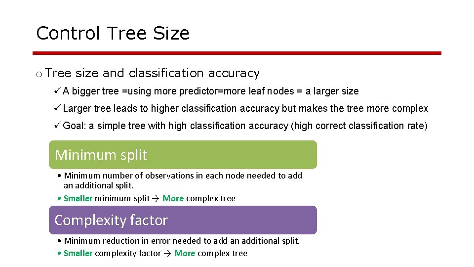
Control Tree Size o Tree size and classification accuracy ü A bigger tree =using more predictor=more leaf nodes = a larger size ü Larger tree leads to higher classification accuracy but makes the tree more complex ü Goal: a simple tree with high classification accuracy (high correct classification rate) Minimum split • Minimum number of observations in each node needed to add an additional split. • Smaller minimum split → More complex tree Complexity factor • Minimum reduction in error needed to add an additional split. • Smaller complexity factor → More complex tree

Clustering Analysis

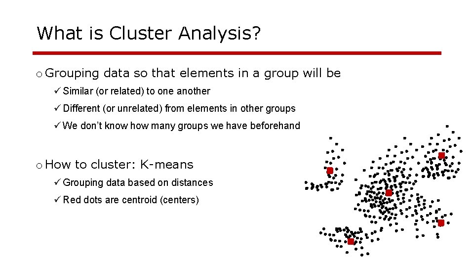
What is Cluster Analysis? o Grouping data so that elements in a group will be ü Similar (or related) to one another ü Different (or unrelated) from elements in other groups ü We don’t know how many groups we have beforehand o How to cluster: K-means ü Grouping data based on distances ü Red dots are centroid (centers)

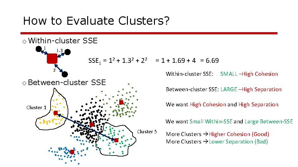
How to Evaluate Clusters? o Within-cluster SSE 1 1. 3 SSE 1 = 12 + 1. 32 + 22 = 1 + 1. 69 + 4 = 6. 69 2 Within-cluster SSE: o Between-cluster SSE SMALL –High Cohesion Between-cluster SSE: LARGE –High Separation We want High Cohesion and High Separation Cluster 1 We want Small Within-SSE and Large Between-SSE Cluster 5 More Clusters Higher Cohesion (Good) More Clusters Lower Separation (Bad)

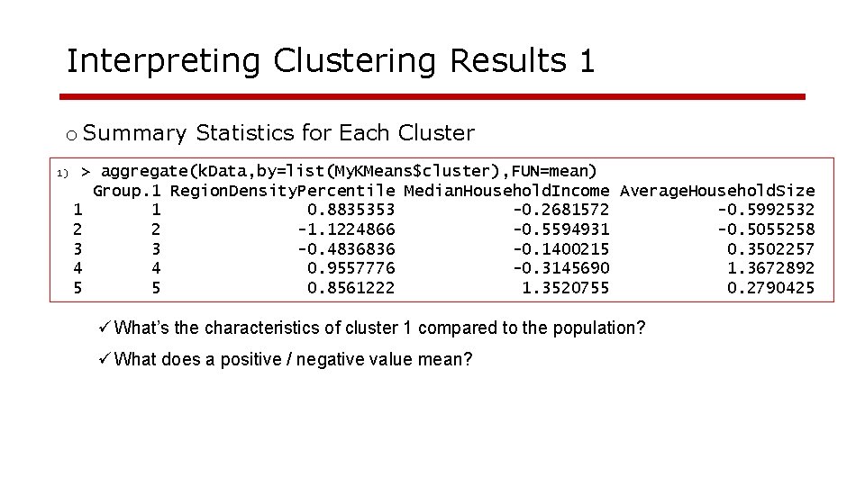
Interpreting Clustering Results 1 o Summary Statistics for Each Cluster 1) > aggregate(k. Data, by=list(My. KMeans$cluster), FUN=mean) Group. 1 Region. Density. Percentile Median. Household. Income Average. Household. Size 1 1 0. 8835353 -0. 2681572 -0. 5992532 2 2 -1. 1224866 -0. 5594931 -0. 5055258 3 3 -0. 4836836 -0. 1400215 0. 3502257 4 4 0. 9557776 -0. 3145690 1. 3672892 5 5 0. 8561222 1. 3520755 0. 2790425 ü What’s the characteristics of cluster 1 compared to the population? ü What does a positive / negative value mean?

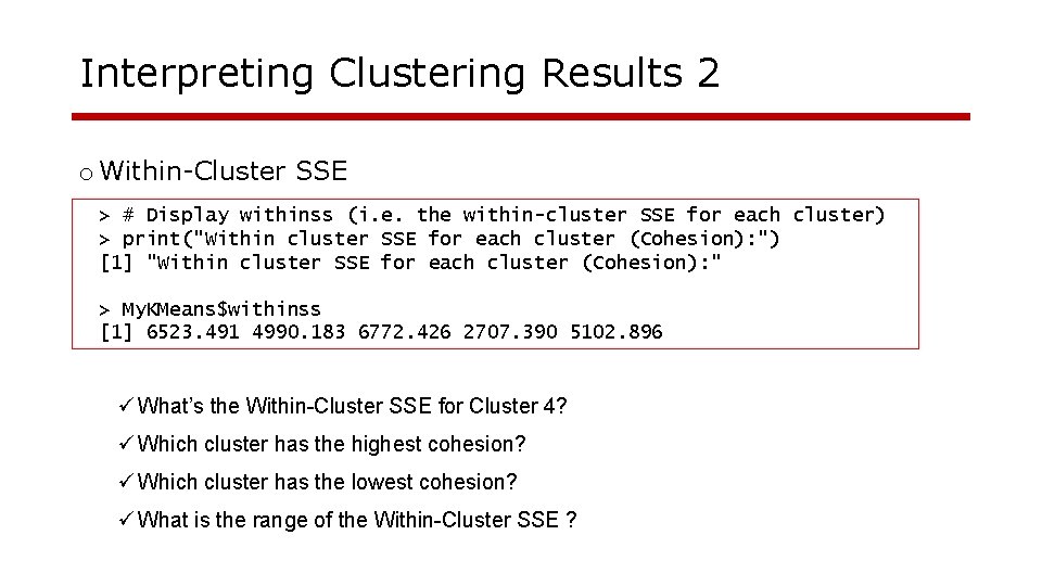
Interpreting Clustering Results 2 o Within-Cluster SSE > # Display withinss (i. e. the within-cluster SSE for each cluster) > print("Within cluster SSE for each cluster (Cohesion): ") [1] "Within cluster SSE for each cluster (Cohesion): " > My. KMeans$withinss [1] 6523. 491 4990. 183 6772. 426 2707. 390 5102. 896 ü What’s the Within-Cluster SSE for Cluster 4? ü Which cluster has the highest cohesion? ü Which cluster has the lowest cohesion? ü What is the range of the Within-Cluster SSE ?

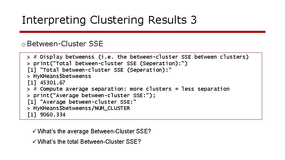
Interpreting Clustering Results 3 o Between-Cluster SSE > # Display betweenss (i. e. the between-cluster SSE between clusters) > print("Total between-cluster SSE (Seperation): ") [1] "Total between-cluster SSE (Seperation): " > My. KMeans$betweenss [1] 45301. 67 > # Compute average separation: more clusters = less separation > print("Average between-cluster SSE: "); [1] "Average between-cluster SSE: " > My. KMeans$betweenss/NUM_CLUSTER [1] 9060. 334 ü What’s the average Between-Cluster SSE? ü What’s the total Between-Cluster SSE?

Association Rules Mining

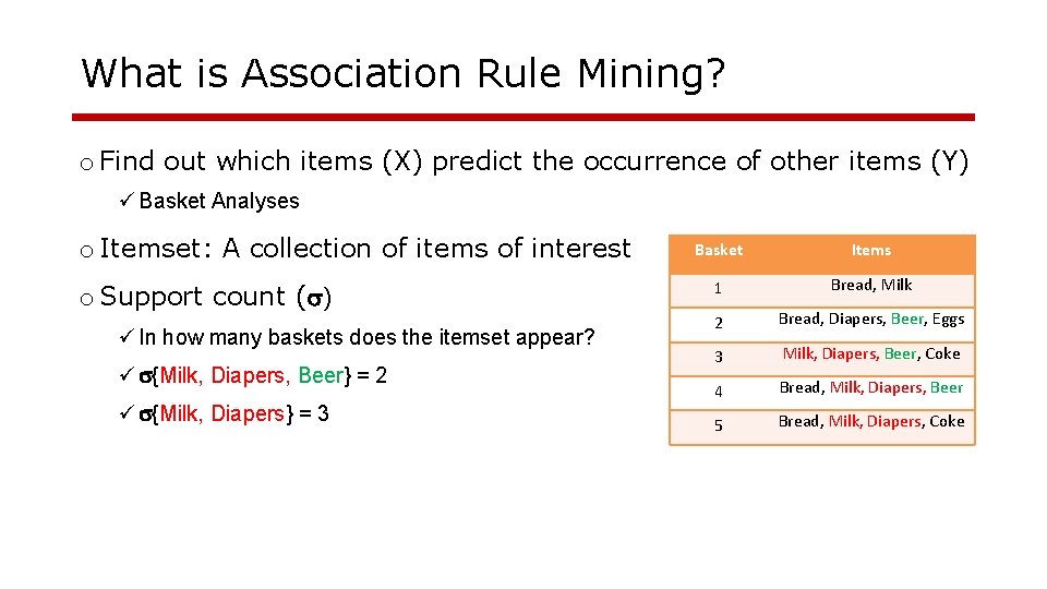
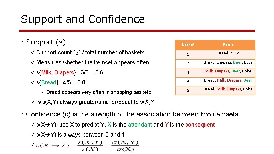
What is Association Rule Mining? o Find out which items (X) predict the occurrence of other items (Y) ü Basket Analyses o Itemset: A collection of items of interest o Support count ( ) ü In how many baskets does the itemset appear? ü {Milk, Diapers, Beer} = 2 ü {Milk, Diapers} = 3 Basket Items 1 Bread, Milk 2 Bread, Diapers, Beer, Eggs 3 Milk, Diapers, Beer, Coke 4 Bread, Milk, Diapers, Beer 5 Bread, Milk, Diapers, Coke

Support and Confidence o Support (s) Basket Items ü Support count ( ) / total number of baskets 1 Bread, Milk ü Measures whether the itemset appears often 2 Bread, Diapers, Beer, Eggs ü s{Milk, Diapers}= 3/5 = 0. 6 3 Milk, Diapers, Beer, Coke ü s{Bread}= 4/5 = 0. 8 4 Bread, Milk, Diapers, Beer 5 Bread, Milk, Diapers, Coke • Bread appears very often in shopping baskets ü Is s(X, Y) always greater/smaller/equal to s(X)? o Confidence (c) is the strength of the association between two itemsets ü c(X Y): use X to predict Y, X is the attendant and Y is the consequent ü c(X Y) is always between 0 and 1 ü

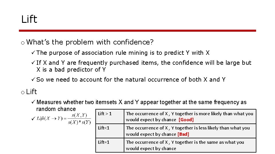
Lift o What’s the problem with confidence? ü The purpose of association rule mining is to predict Y with X ü If X and Y are frequently purchased items, the confidence will be large but X is a bad predictor of Y ü So we need to account for the natural occurrence of both X and Y o Lift ü Measures whether two itemsets X and Y appear together at the same frequency as random chance ü Lift > 1 The occurrence of X , Y together is more likely than what you would expect by chance [Good] Lift<1 The occurrence of X , Y together is less likely than what you would expect by chance [Bad] Lift=1 The occurrence of X , Y together is the same as what you would expect by chance

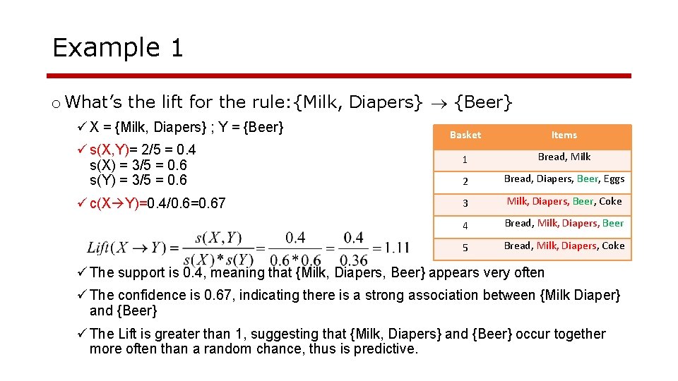
Example 1 o What’s the lift for the rule: {Milk, Diapers} {Beer} ü X = {Milk, Diapers} ; Y = {Beer} ü s(X, Y)= 2/5 = 0. 4 s(X) = 3/5 = 0. 6 s(Y) = 3/5 = 0. 6 ü c(X Y)=0. 4/0. 6=0. 67 Basket Items 1 Bread, Milk 2 Bread, Diapers, Beer, Eggs 3 Milk, Diapers, Beer, Coke 4 Bread, Milk, Diapers, Beer 5 Bread, Milk, Diapers, Coke ü The support is 0. 4, meaning that {Milk, Diapers, Beer} appears very often ü The confidence is 0. 67, indicating there is a strong association between {Milk Diaper} and {Beer} ü The Lift is greater than 1, suggesting that {Milk, Diapers} and {Beer} occur together more often than a random chance, thus is predictive.

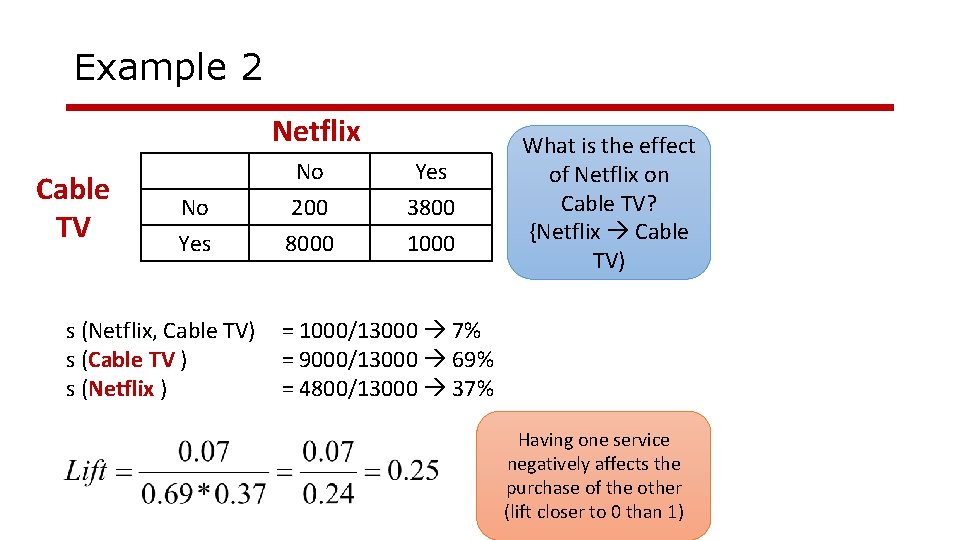
Example 2 Netflix Cable TV No Yes s (Netflix, Cable TV) s (Cable TV ) s (Netflix ) No 200 8000 Yes 3800 1000 What is the effect of Netflix on Cable TV? {Netflix Cable TV) = 1000/13000 7% = 9000/13000 69% = 4800/13000 37% Having one service negatively affects the purchase of the other (lift closer to 0 than 1)

Good Luck!