Essentials of EconomicsMacroeconomics Prof KJ Sung Fall of

Essentials of Economics-Macroeconomics Prof. KJ Sung Fall of 2018 1

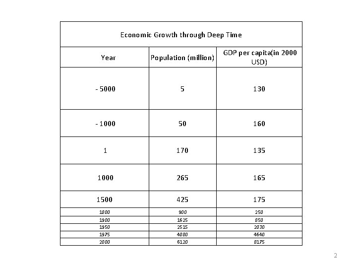
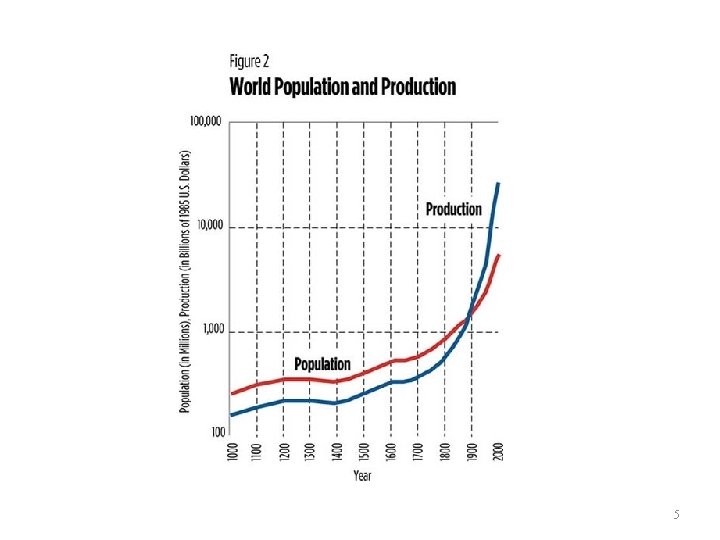
Economic Growth through Deep Time 　Year Population (million) GDP per capita(in 2000 USD) - 5000 5 130 - 1000 50 160 1 170 135 1000 265 1500 425 175 1800 1950 1975 2000 900 1625 2515 4080 6120 250 850 2030 4640 8175 2

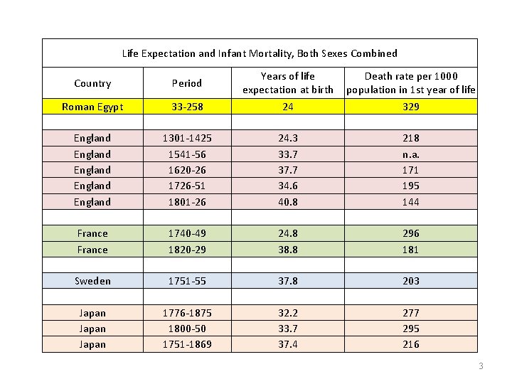
Life Expectation and Infant Mortality, Both Sexes Combined Country Roman Egypt 　 England England 　 France 　 Sweden 　 Japan Period　 33 -258 　 1301 -1425 1541 -56 1620 -26 1726 -51 1801 -26 　 1740 -49 1820 -29 　 1751 -55 　 1776 -1875 1800 -50 1751 -1869 Years of life expectation at birth 24 　 24. 3 33. 7 37. 7 34. 6 40. 8 　 24. 8 38. 8 　 37. 8 　 32. 2 33. 7 37. 4 Death rate per 1000 population in 1 st year of life 329 　 218 n. a. 171 195 144 　 296 181 　 203 　 277 295 216 3

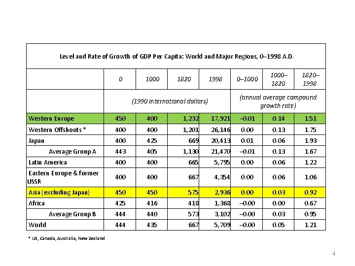
Level and Rate of Growth of GDP Per Capita: World and Major Regions, 0– 1998 A. D. 0 　 1000 1820 1998 0– 1000– 1820– 1998 (annual average compound growth rate) (1990 international dollars) Western Europe 450 400 1, 232 17, 921 – 0. 01 0. 14 1. 51 Western Offshoots * 400 1, 201 26, 146 0. 00 0. 13 1. 75 Japan 400 425 669 20, 413 0. 01 0. 06 1. 93 443 405 1, 130 21, 470 – 0. 01 0. 13 1. 67 Latin America 400 665 5, 795 0. 00 0. 06 1. 22 Eastern Europe & former USSR 400 667 4, 354 0. 00 0. 06 1. 06 Asia (excluding Japan) 450 575 2, 936 0. 00 0. 03 0. 92 Africa 425 416 418 1, 368 – 0. 00 0. 67 444 440 573 3, 102 – 0. 00 0. 03 0. 95 444 435 667 5, 709 – 0. 00 0. 05 1. 21 Average Group A Average Group B World * US, Canada, Australia, New Zealand 4

5

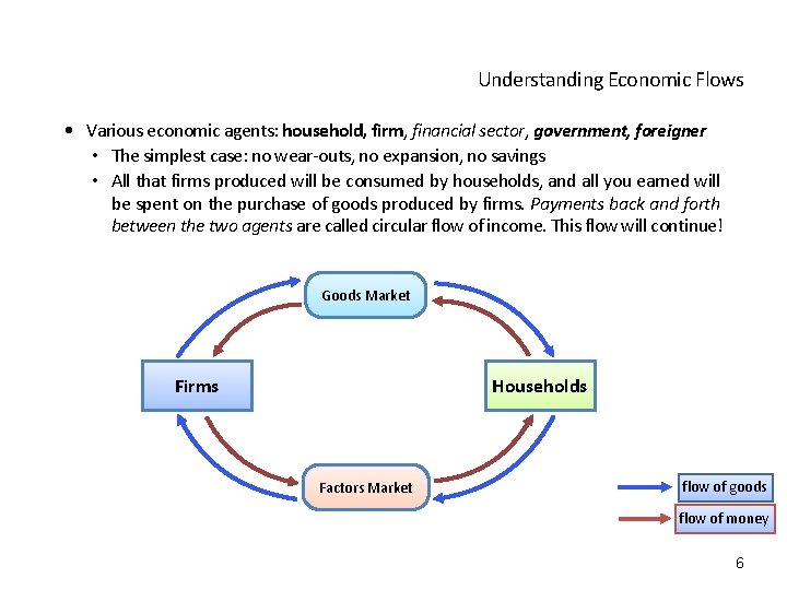
Understanding Economic Flows • Various economic agents: household, firm, financial sector, government, foreigner • The simplest case: no wear-outs, no expansion, no savings • All that firms produced will be consumed by households, and all you earned will be spent on the purchase of goods produced by firms. Payments back and forth between the two agents are called circular flow of income. This flow will continue! Goods Market Firms Households Factors Market flow of goods flow of money 6

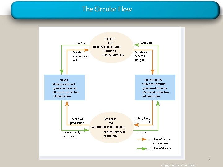
The Circular Flow Revenue Goods and services sold MARKETS FOR GOODS AND SERVICES • Firms sell • Households buy Wages, rent, and profit Goods and services bought HOUSEHOLDS • Buy and consume goods and services • Own and sell factors of production FIRMS • Produce and sell goods and services • Hire and use factors of production Factors of production Spending MARKETS FOR FACTORS OF PRODUCTION • Households sell • Firms buy Labor, land, and capital Income = Flow of inputs and outputs = Flow of dollars Principles of Economics 2016 7 Copyright © 2004 South-Western

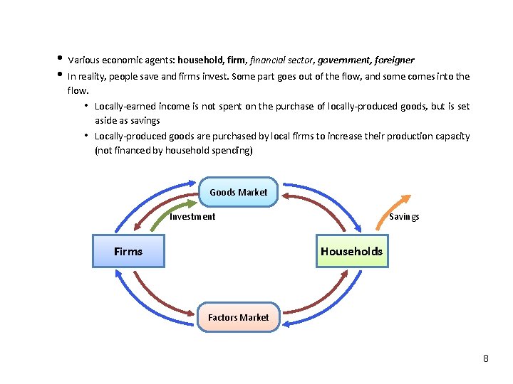
• Various economic agents: household, firm, financial sector, government, foreigner • In reality, people save and firms invest. Some part goes out of the flow, and some comes into the flow. • Locally-earned income is not spent on the purchase of locally-produced goods, but is set aside as savings • Locally-produced goods are purchased by local firms to increase their production capacity (not financed by household spending) Goods Market Investment Firms Savings Households Factors Market 8

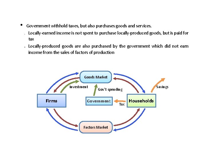
• Government withhold taxes, but also purchases goods and services. Locally-earned income is not spent to purchase locally-produced goods, but is paid for tax Locally-produced goods are also purchased by the government which did not earn income from the sales of factors of production Goods Market Investment Firms Savings Gov’t spending Government Factors Market Tax Households

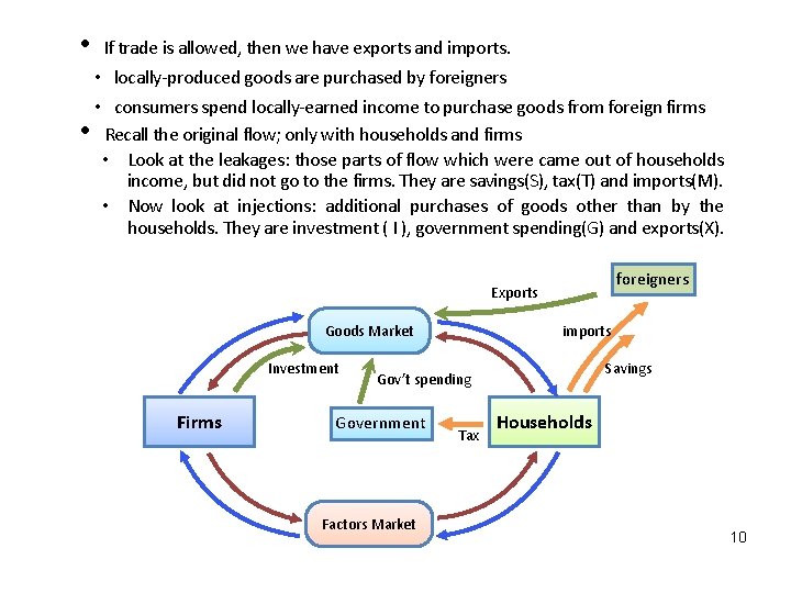
• If trade is allowed, then we have exports and imports. • locally-produced goods are purchased by foreigners • consumers spend locally-earned income to purchase goods from foreign firms • Recall the original flow; only with households and firms • Look at the leakages: those parts of flow which were came out of households income, but did not go to the firms. They are savings(S), tax(T) and imports(M). • Now look at injections: additional purchases of goods other than by the households. They are investment ( I ), government spending(G) and exports(X). foreigners Exports imports Goods Market Investment Firms Savings Gov’t spending Government Factors Market Tax Households 10

Circular Flow of Income • How do we measure the size of an economy? Size of economic activity? • • • Three ways to measure the size of flow. First, concentrate on the production side. Who produced how much? Second, income side. How much earned? Third, expenditure side. How much each agent spent? Who purchases goods? If something was produced, during the production, income must have been accrued (including profit), and all income must have been spent. • Output method: rather easy to calculate and most accurate, but watch out for double counting • Income method is the least accurate. Those income only in return for productive services is included. • Expenditure method should include those on final goods. Note that investment includes inventory investment. There are expenditures by firms (investment), by households (consumption), by government (government spending), and by foreigners (net export). 11

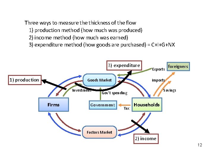
Three ways to measure thickness of the flow 1) production method (how much was produced) 2) income method (how much was earned) 3) expenditure method (how goods are purchased) = C+I+G+NX 3) expenditure 1) production Firms Savings Gov’t spending Government foreigners imports Goods Market Investment Exports Tax Households Factors Market 2) income 12

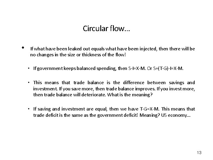
Circular flow… • If what have been leaked out equals what have been injected, then there will be no changes in the size or thickness of the flow! • If government keeps balanced spending, then S-I=X-M. Or S+(T-G)-I=X-M. • This means that trade balance is the difference between savings and investment. If you save more, then trade balance improves. If you invest more, then trade balance will deteriorate. What is the meaning? • If saving and investment are equal, then we have T-G=X-M. This means that trade deficit is the same as the government deficit! Meaning? US economy… 13

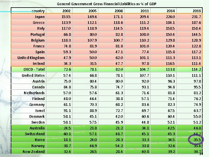
General Government Gross Financial Liabilities as % of GDP country Japan Greece Italy Portugal Belgium France Spain United Kingdom Ireland OECD - Total United States Austria Canada Netherlands Finland Germany Israel Denmark Sweden Australia Switzerland Korea Norway New Zealand 2002 153. 5 113. 9 117. 0 66. 8 118. 3 74. 8 59. 3 47. 9 34. 3 72. 6 57. 4 75. 0 84. 8 57. 0 48. 0 61. 1 91. 1 58. 1 24. 5 60. 1 18. 1 38. 7 32. 4 2005 169. 6 112. 1 118. 9 80. 0 107. 9 81. 9 50. 0 31. 5 78. 1 66. 8 80. 4 75. 8 57. 6 46. 4 70. 3 88. 9 45. 1 57. 5 21. 8 57. 1 24. 0 46. 9 26. 5 2008 171. 1 118. 6 114. 5 82. 8 100. 7 81. 8 47. 1 62. 0 47. 7 82. 0 78. 1 80. 0 74. 7 61. 3 38. 8 68. 2 72. 7 42. 0 45. 9 21. 2 48. 7 28. 3 54. 2 28. 4 2011 209. 4 111. 2 119. 4 108. 0 110. 2 101. 0 77. 4 101. 1 97. 8 104. 7 107. 7 92. 0 93. 1 71. 6 57. 1 83. 6 69. 7 60. 6 44. 8 34. 1 45. 1 33. 3 33. 8 40. 8 2014 226. 0 184. 1 158. 5 150. 4 129. 8 120. 4 115. 8 111. 3 116. 5 113. 8 110. 1 96. 3 94. 8 81. 8 71. 4 82. 3 67. 5 60. 4 52. 1 42. 5 45. 3 34. 5 32. 6 39. 2 2016 231. 7 187. 6 158. 4 144. 5 128. 9 122. 8 117. 2 113. 1 111. 4 114. 2 111. 1 97. 8 95. 5 81. 2 76. 2 74. 9 63. 7 55. 0 51. 2 46. 8 44. 7 35. 5 35. 4 34. 7 14

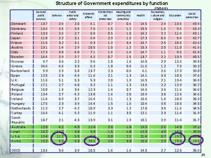
General public services Structure of Government expenditures by function (2011) Public Environmen Housing and Recreation, Defence order and safety Economic affairs tal protection community amenities Health culture and religion Education Social protection Denmark Germany Finland Japan France Austria Italy Sweden Norway Greece Switzerland Spain U. K. Portugal Belgium Poland Ireland Hungary Netherlands Turkey Czech Republic Australia Israel U. S. A. Korea 13. 7 13. 6 13. 3 11. 0 11. 5 13. 1 17. 3 14. 4 9. 7 24. 6 9. 9 12. 5 11. 6 17. 1 15. 0 13. 4 11. 4 17. 5 11. 2 16. 4 2. 6 2. 2 3. 2 1. 4 3. 0 2. 9 3. 6 4. 6 2. 9 2. 3 5. 1 2. 7 1. 8 2. 7 0. 9 2. 3 2. 7 4. 1 2. 0 3. 5 2. 7 3. 1 2. 9 4. 0 2. 7 2. 2 3. 3 5. 0 4. 8 5. 3 4. 0 3. 4 4. 2 3. 7 3. 9 4. 2 5. 2 6. 1 7. 8 8. 8 9. 8 6. 3 10. 5 7. 1 8. 2 9. 6 6. 2 13. 7 11. 6 5. 3 8. 2 12. 3 13. 0 16. 4 14. 4 10. 9 11. 9 0. 7 1. 5 0. 5 2. 9 1. 0 1. 8 0. 7 1. 5 1. 0 2. 3 2. 1 2. 0 1. 1 1. 4 1. 6 2. 1 1. 5 3. 3 1. 1 0. 6 1. 2 1. 0 1. 8 3. 4 1. 2 1. 4 1. 5 1. 6 0. 4 0. 6 1. 3 1. 8 1. 3 0. 7 2. 0 1. 3 1. 6 1. 2 3. 5 14. 5 15. 5 14. 2 17. 3 14. 7 15. 3 14. 7 13. 7 16. 5 11. 6 6. 1 14. 1 16. 5 13. 8 14. 8 10. 9 15. 6 10. 4 17. 0 12. 1 2. 8 1. 8 2. 2 0. 8 2. 5 2. 0 1. 1 2. 2 2. 9 1. 2 2. 6 3. 3 2. 1 2. 2 2. 4 3. 0 1. 8 3. 5 2. 3 13. 5 9. 4 11. 6 8. 4 10. 8 11. 0 8. 5 13. 3 12. 6 7. 9 10. 5 13. 4 12. 9 11. 6 12. 8 10. 9 10. 5 11. 6 11. 4 43. 8 43. 3 43. 1 42. 7 42. 6 41. 0 40. 5 39. 8 39. 3 39. 0 37. 4 36. 8 36. 7 36. 6 35. 9 34. 5 31. 9 10. 7 2. 1 4. 3 13. 9 3. 1 1. 9 18. 1 2. 9 11. 4 31. 7 12. 5 14. 7 12. 4 15. 2 4. 1 14. 7 11. 7 8. 6 4. 8 3. 8 5. 5 4. 2 11. 4 5. 8 9. 4 20. 1 2. 6 1. 5 0. 0 2. 4 1. 8 1. 0 2. 1 3. 3 19. 2 12. 3 21. 4 15. 2 2. 1 3. 9 0. 7 2. 2 14. 5 16. 5 15. 8 27. 1 25. 9 21. 3 13. 1 OECD 13. 6 3. 9 10. 5 1. 6 Kor. Econ. Dev 1. 6 14. 5 2. 7 12. 5 35. 6 15

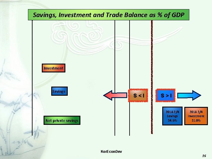
Savings, Investment and Trade Balance as % of GDP Investment Savings S<I S>I 2018 2/4 Savings 34. 6% Net private savings Kor. Econ. Dev 2018 2/4 Investment 31. 0% 16

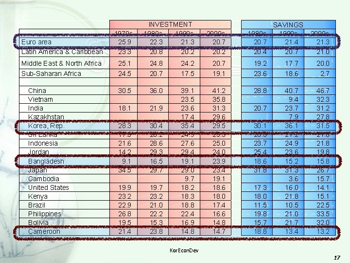
INVESTMENT 1980 s 1990 s 22. 3 21. 3 20. 8 20. 2 Euro area Latin America & Caribbean 1970 s 25. 9 23. 3 Middle East & North Africa 25. 1 24. 8 24. 2 20. 7 19. 2 17. 7 20. 0 Sub-Saharan Africa 24. 5 30. 5 18. 1 28. 3 17. 5 21. 6 14. 2 9. 1 34. 5 19. 9 23. 2 22. 9 26. 8 19. 5 21. 4 20. 7 36. 0 21. 9 30. 4 26. 2 28. 6 29. 3 16. 5 29. 7 19. 7 23. 2 21. 0 22. 2 15. 3 23. 8 17. 5 39. 1 23. 5 23. 6 17. 4 35. 4 24. 9 27. 6 29. 4 19. 1 29. 0 9. 7 18. 2 18. 3 18. 8 22. 4 16. 9 14. 8 19. 1 41. 2 35. 8 31. 3 29. 6 29. 5 25. 3 25. 0 24. 0 23. 9 23. 4 19. 1 18. 6 18. 0 17. 4 16. 6 14. 8 14. 7 23. 6 28. 8 20. 7 30. 1 20. 3 23. 7 25. 4 18. 6 31. 8 17. 3 18. 0 11. 5 19. 8 15. 7 18. 8 18. 6 40. 7 9. 4 23. 7 7. 9 36. 1 21. 2 24. 9 23. 6 15. 2 31. 3 3. 6 16. 0 21. 8 10. 5 21. 0 21. 7 13. 4 2. 7 46. 7 32. 3 31. 2 27. 8 31. 5 21. 8 19. 8 15. 8 26. 7 15. 7 14. 1 15. 1 22. 5 33. 5 32. 0 13. 2 China Vietnam India Kazakhstan Korea, Rep. Sri Lanka Indonesia Jordan Bangladesh Japan Cambodia United States Kenya Brazil Philippines Bolivia Cameroon Kor. Econ. Dev 2000 s 20. 7 20. 2 SAVINGS 1980 s 1990 s 20. 7 21. 4 20. 7 2000 s 21. 3 21. 0 17

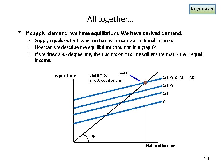
Circular Flow…(cont’d) • Another notion of equilibrium: supply = demand. • What constitutes supply? Output is supply (and equals income) • What constitutes demand? Who demands this output? Households(C), firms(I), government(G), and foreigners(X-M). • Thus demand is composed of C+I+G+(X-M). This is the same as aggregate expenditures. • Thus, if we denote Y as output, then Supply=Demand ➔Y=C+ I +G+NX. • Was it not an identity? Yes, it was true, ex-post. (Y ≡ C+ I +G+NX) • But, not here; we mean, ex-ante. Difference is in inventory investment. • Keep in mind: S+T+M = I+G+X, and/or Y = C+I+G+(X-M) 18

National Income Determination • How is national income determined? There are basically two different views. • Keynesian view: largely determined by the level of aggregate demand(AG), and AG can be adjusted through fiscal policy (affecting T and G). • Monetarist view: controlling demand is important, but basically leave them alone (no fiscal policy, and just stable money growth). • Both schools stress the importance of demand management. • What about supply? Supply is basically total output. • What constitutes demand? • Consumption, investment and government expenditure. And net export. • If we denote Y as output, then Supply=Demand ➔Y=C+I+G+NX. 19

Keynesian Original Keynesian Approach • Consumption demand • This takes up the largest portion of demand, and is quite stable. • What determines consumption demand? Disposable income, consumer confidence, wealth of consumers, tax and so on. • We assume for the moment that consumption only depends on income. We also assume there are no taxes. • If factors other than income changes, then the consumption curve will shift. • How much do you spend and save? Let’s introduce a concept of marginal propensity to consume (mpc). It is the ratio of consumption to the increased income. We also assume mpc is constant, and less than 1. • There are many theories how consumption is determined. You may not decide consumption based on your current income. But these alternative theories are not satisfactory either, and they do not change our analysis much. Thus, we assume consumption depends on income only, and mpc is constant. 20

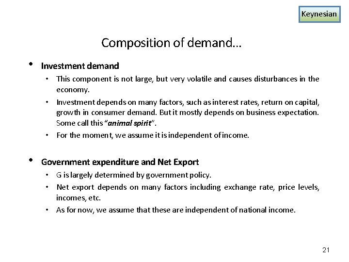
Keynesian Composition of demand… • Investment demand • This component is not large, but very volatile and causes disturbances in the economy. • Investment depends on many factors, such as interest rates, return on capital, growth in consumer demand. But it mostly depends on business expectation. Some call this “animal spirit”. • For the moment, we assume it is independent of income. • Government expenditure and Net Export • G is largely determined by government policy. • Net export depends on many factors including exchange rate, price levels, incomes, etc. • As for now, we assume that these are independent of national income. 21

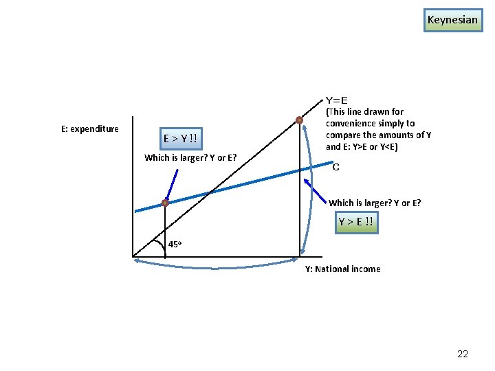
Keynesian E: expenditure E > Y !! Which is larger? Y or E? Y=E (This line drawn for convenience simply to compare the amounts of Y and E: Y>E or Y<E) C Which is larger? Y or E? Y > E !! 45 o Y: National income 22

Keynesian All together… • If supply=demand, we have equilibrium. We have derived demand. • Supply equals output, which in turn is the same as national income. • How can we describe the equilibrium condition in a graph? • If we draw a 45 degree line, then points on this line will ensure that AD will equal income. expenditure Y=AD Since Y=S, S=AD: equilibrium!! C+I+G+(X-M) = AD C+I+G C+I C 45 o National income 23

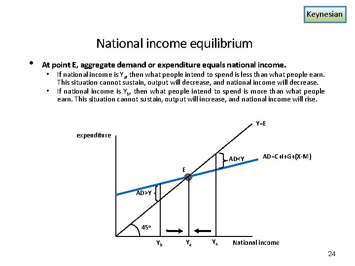
Keynesian National income equilibrium • At point E, aggregate demand or expenditure equals national income. • • If national income is Ya, then what people intend to spend is less than what people earn. This situation cannot sustain, output will decrease, and national income will decrease. If national income is Yb, then what people intend to spend is more than what people earn. This situation cannot sustain, output will increase, and national income will rise. Y=E expenditure AD<Y AD=C+I+G+(X-M) E AD>Y 45 o Yb Ye Ya National income 24

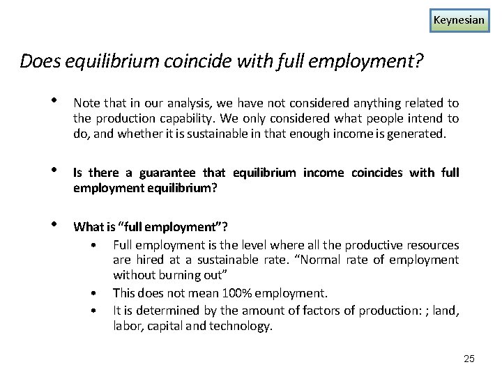
Keynesian Does equilibrium coincide with full employment? • Note that in our analysis, we have not considered anything related to the production capability. We only considered what people intend to do, and whether it is sustainable in that enough income is generated. • Is there a guarantee that equilibrium income coincides with full employment equilibrium? • What is “full employment”? • Full employment is the level where all the productive resources are hired at a sustainable rate. “Normal rate of employment without burning out” • This does not mean 100% employment. • It is determined by the amount of factors of production: ; land, labor, capital and technology. 25

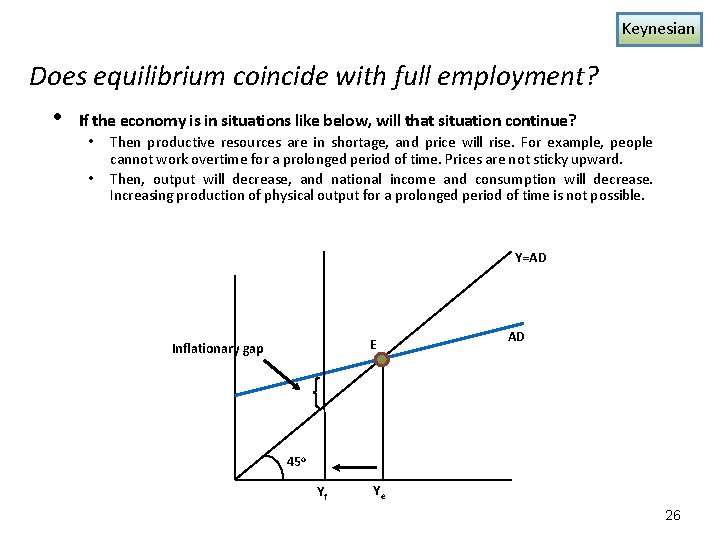
Keynesian Does equilibrium coincide with full employment? • If the economy is in situations like below, will that situation continue? • • Then productive resources are in shortage, and price will rise. For example, people cannot work overtime for a prolonged period of time. Prices are not sticky upward. Then, output will decrease, and national income and consumption will decrease. Increasing production of physical output for a prolonged period of time is not possible. Y=AD E Inflationary gap AD 45 o Yf Ye 26

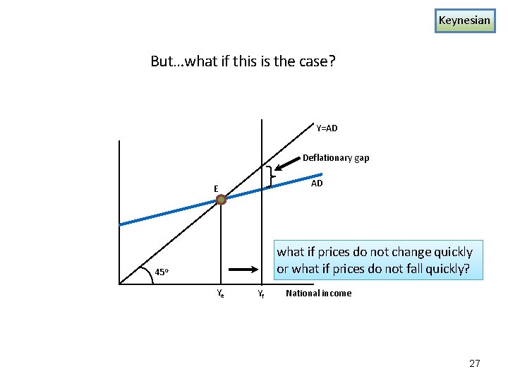
Keynesian But…what if this is the case? Y=AD Deflationary gap AD E what if prices do not change quickly or what if prices do not fall quickly? 45 o Ye Yf National income 27

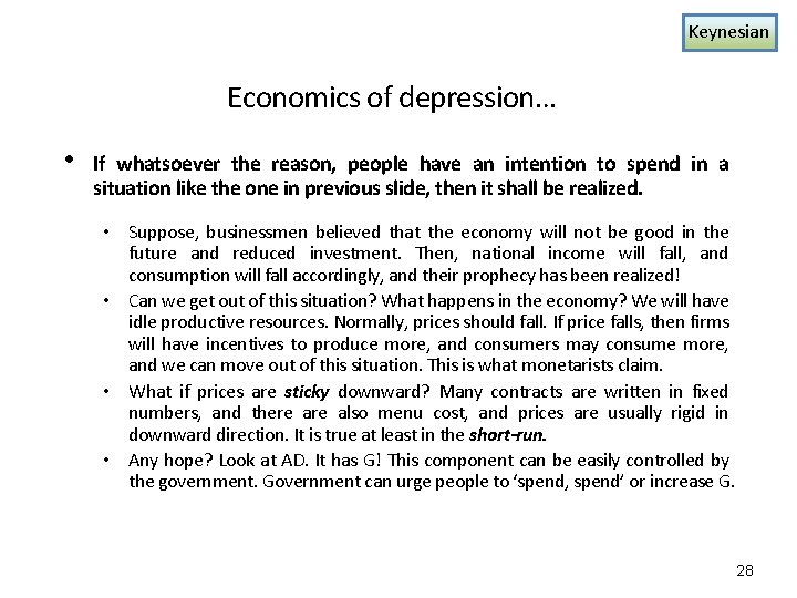
Keynesian Economics of depression… • If whatsoever the reason, people have an intention to spend in a situation like the one in previous slide, then it shall be realized. • Suppose, businessmen believed that the economy will not be good in the future and reduced investment. Then, national income will fall, and consumption will fall accordingly, and their prophecy has been realized! • Can we get out of this situation? What happens in the economy? We will have idle productive resources. Normally, prices should fall. If price falls, then firms will have incentives to produce more, and consumers may consume more, and we can move out of this situation. This is what monetarists claim. • What if prices are sticky downward? Many contracts are written in fixed numbers, and there also menu cost, and prices are usually rigid in downward direction. It is true at least in the short-run. • Any hope? Look at AD. It has G! This component can be easily controlled by the government. Government can urge people to ‘spend, spend’ or increase G. 28

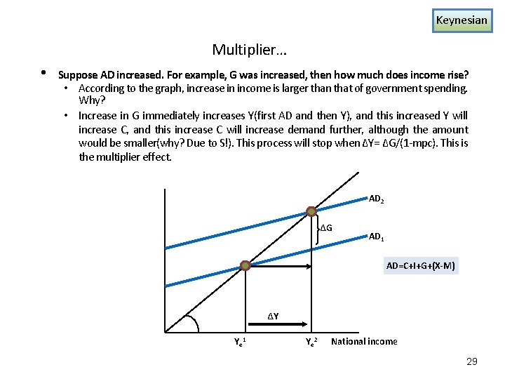
Keynesian Multiplier… • Suppose AD increased. For example, G was increased, then how much does income rise? • According to the graph, increase in income is larger than that of government spending. Why? • Increase in G immediately increases Y(first AD and then Y), and this increased Y will increase C, and this increase C will increase demand further, although the amount would be smaller(why? Due to S!). This process will stop when ΔY= ΔG/(1 -mpc). This is the multiplier effect. AD 2 ΔG AD 1 AD=C+I+G+(X-M) ΔY Ye 1 Ye 2 National income 29

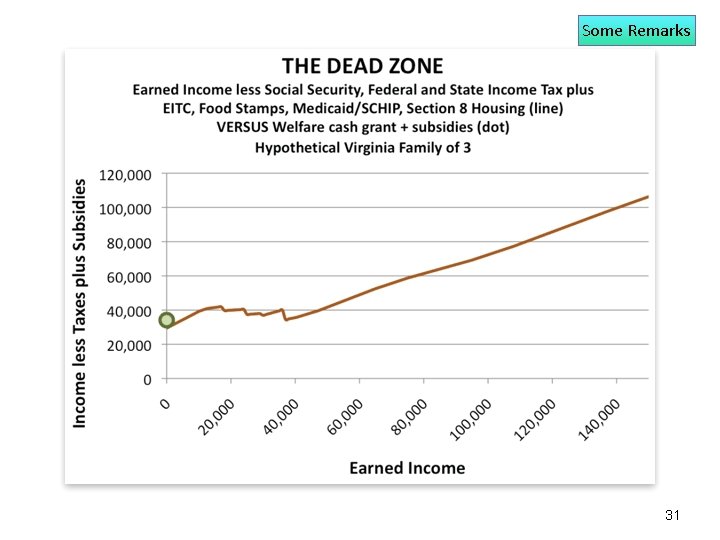
Some Remarks on Fiscal Policy • Fiscal policy is a discretionary one. • Limitations of fiscal policy • Topics in taxation • But in the economy, we have also automatic stabilizer (sometimes called built-in stabilizer). Tax revenue and welfare benefits are examples. • In the real world, tax rate is fixed, not the total amount of tax, T. • • • Takes a long time to implement and some projects are long-term Difficult to reverse: ratchet effect Escalation of costs General tendency of rising taxes, not reducing taxes. In general, we have moral hazard problem: emergence of public choice theory • Direct taxes are equitable, automatic stabilizers, less inflationary: poverty trap, and fiscal drag • Indirect taxes are regressive, but gives choices to the consumer. Also quick and immediate effect, but inflationary. 30

Some Remarks 31

Monetarist Monetary Policy: the essence • • • Monetarists basically believes in the market functioning, and output can be increased only through expanded productive efficiency. • Short-run adjustment will bring in disturbance, not adjustment. If sufficient time and flexibility is given, the economy will reach full employment equilibrium. • Keynesians maintain that there is not enough flexibility in prices, and “in the long-run, we may be all dead. ” Excessive government spending entails budget deficits, and may end up printing money, which causes inflation. • More money will increase aggregate demand, and accordingly inflation. This process will also fuel expectations of future inflation: wage-price spiral. In short, unemployment can be reduced in the longer term only if inflationary expectations are diminished. 32

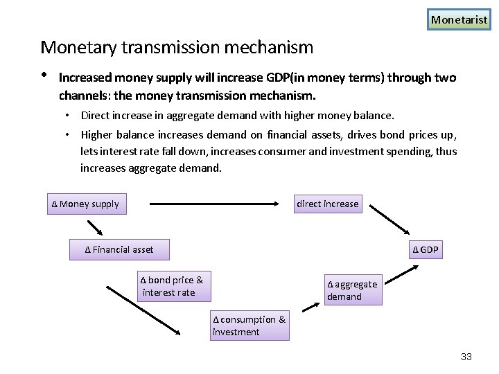
Monetarist Monetary transmission mechanism • Increased money supply will increase GDP(in money terms) through two channels: the money transmission mechanism. • Direct increase in aggregate demand with higher money balance. • Higher balance increases demand on financial assets, drives bond prices up, lets interest rate fall down, increases consumer and investment spending, thus increases aggregate demand. Δ Money supply direct increase Δ GDP Δ Financial asset Δ bond price & interest rate Δ aggregate demand Δ consumption & investment 33

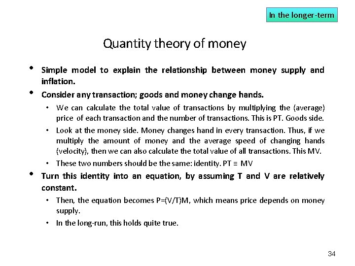
In the longer-term Quantity theory of money • • • Simple model to explain the relationship between money supply and inflation. Consider any transaction; goods and money change hands. • We can calculate the total value of transactions by multiplying the (average) price of each transaction and the number of transactions. This is PT. Goods side. • Look at the money side. Money changes hand in every transaction. Thus, if we multiply the amount of money and the average speed of changing hands (velocity), then we can also calculate the total value of all transactions. This MV. • These two numbers should be the same: identity. PT ≡ MV Turn this identity into an equation, by assuming T and V are relatively constant. • Then, the equation becomes P=(V/T)M, which means price depends on money supply. • In the long-run, this holds quite true. 34

Definition and creation of money • • Liquidity spectrum: money, near money, quasi-money… Banks create money. • Not all the money deposited in the banks are withdrawn, and banks can lend this reserve. This lending will be deposited, and banks can further lend out reserves. Lion’s share of money supply is from banks. Bank credit multiplier: 1/(reserve ratio). (7% in Korea as of 2011) • How to control money supply? Mainly through buying and selling securities. • If government purchases securities(mostly bonds), then money supply will increase. • If government sells securities, then money supply contracts. (If government spends the proceeds, then there will be no change in money supply) • This is open market operation. 35

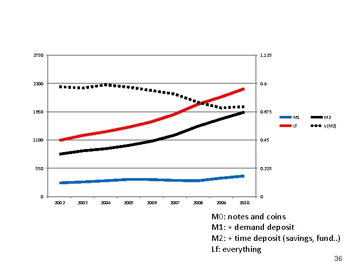
2750 1. 125 2200 0. 9 1650 0. 675 1100 0. 45 550 0. 225 0 M 1 M 2 Lf V(M 2) 0 2002 2003 2004 2005 2006 2007 2008 2009 2010 M 0: notes and coins M 1: + demand deposit M 2: + time deposit (savings, fund. . ) Lf: everything 36

Government borrowing • • • How does government finance their borrowing? • Borrowing from the private sector: not much change in money supply. • Borrowing from the bank: creates multiple effect in money supply. Those idle money in the banks is now fed back into the economy. If government wants to expand spending, but not the money supply, then government has to borrow from non-banking sector. • But, then government has to compete with private sector, and may crowd out private investment. Can the government buy and sell securities as they wish? What are the instrument? • The price of securities is interest rate. By controlling interest rates, government control money supply, and aggregate demand. • In many developed countries, interest rate is the major instrument in controlling the aggregate demand. Fiscal policies are not widely used, as they are mostly running budget deficit, and also because of its ratchet effect. 37

In the shorter-term Closer look at monetarists… • • • Criticisms of monetarists, first on quantity theory of money. • Does M cause P to change or the other way around? • Are V and T stable? If the economy is not at full employment, then T is not fixed, and V is not stable as assumed. Then, money transmission mechanism. Are relationships strong? • Δ M and Δ r; and Δ r and Δ AD Let’s consider demand for money, and the impact of interest rate on investment. • If interest rate is higher, then people will hold smaller amount of money. But interest rate may not affect money demand much: insensitive to interest rate. • Considerable debates were held without conclusion. In general, demand seems inelastic if interest rates are higher, and elastic if rates are lower. • Keynesians argue that the demand is elastic. 38

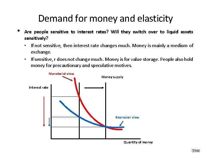
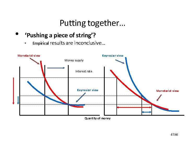
Demand for money and elasticity • Are people sensitive to interest rates? Will they switch over to liquid assets sensitively? • If not sensitive, then interest rate changes much. Money is mainly a medium of exchange. • If sensitive, r does not change much. Money is for value storage. People also hold money for precautionary and speculative motives. Monetarist view Money supply Interest rate Keynesian view Quantity of money 39

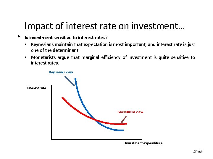
• Impact of interest rate on investment… Is investment sensitive to interest rates? • Keynesians maintain that expectation is most important, and interest rate is just one of the determinant. • Monetarists argue that marginal efficiency of investment is quite sensitive to interest rates. Keynesian view Interest rate Monetarist view Investment expenditure 40

• Putting together… ‘Pushing a piece of string’? • Empirical results are inconclusive… Monetarist view Keynesian view Money supply Interest rate Keynesian view Monetarist view Quantity of money 41

Effects of monetary policy… • • • From a longer-term perspective and with strong government, monetarist policy may work. • Firms will become ‘leaner and fitter’, if they can survive. High interest rates, however, may result in high unemployment in between. • Reduced tax receipts, pressure to reduced public expenditure, reduced investment and economic growth are hard to bear. • Also, high interest rates will result in high exchange rate, and trade balance will deteriorate. • Some firms will borrow even more to solve cash-flow difficulties; distress borrowing. Hard to find a good measure for money supply, hard to sustain high interest rates over long periods. • Also, in many incidences, interest rate policy concerns more with exchange rates; mostly reactionary, and too little, too late. • Recent years have seen proactive policy, like ABS brake system. 42

Exchange Rate Policy • Three exchange rate systems: floating, fixed, and managed. • Appreciation and depreciation: if demand is large and local currency becomes expensive, we say it appreciates. Depreciation is likewise defined. Up or low? • Floating exchange rate: supply and demand determines exchange rate. Supply comes from import, and demand from export, as we pay and receive local currency. They also come from capital transactions. • Fixed exchange rate: if demand is large, then buy hard currencies and provide more local currency. If demand is low, sell hard currencies, and receive local currency. • Managed exchange rate: dirty floating and joint floating. Dirty floating involves arbitrary intervention by the government. Joint floating (snake) pegs values of several currencies against each other. ECU was the most prominent example (now, we have euro). 43

History of world exchange rate system • Two gold standards until 30 s and 70 s. • Gold standard system: internally, money supply was broadly determined by the amount of gold, and international trade was primarily financed by gold shipments. • It was a very stable system and achieved a high degree of automatic balance. • The system broke down due to downward rigidity of price during the interwar period. • Bretton Woods system: lessons from ‘beggar thy neighbor’ policies. US dollar was convertible to gold at fixed rate. From gold to guarantee of gold. • Increasing international liquidity and weakening of US dollar forced US to abandon this system in early 70 s. • Since then, most developed countries rely on floating exchange rate system, usually in the form of managed floating. 44

Determination of exchange rates • Other important determinants of exchange rates: inflation and interest rates • Purchasing power parity: other things equal, different rates of inflation cause changes in exchange rates. If inflation is relatively higher, then local currency will depreciate, since the same amount of money should be able to purchase the same amount of products. Limitations to this explanations come from transportation costs, existence of non-trade goods, and capital flows. • Strong link exists between interest rates and exchange rates. If interest rates are higher, then foreign capital will flow into the country. This inflow increases the demand for local currency, and drives up exchange rates. This link is reinforced by the forward exchange market: you eliminate uncertainty from changes in exchange rates. • Speculation in foreign exchange markets may or may not stabilize the markets. If the magnitude is small, and expectation is in the other direction, then speculation may stabilize the market. If not, then speculation may amplify the variation. In some cases, only rumors may have self-fulfilling prophecy. 45

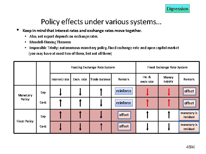
Digression Fixed exchange rates • • Domestic economy is directly linked to the world economy. • If there is depression in the world and price level falls, the export demand decreases, and local economy contracts, too. • Basically, this system works as a discipline to the local policy makers. Managing exchange rates requires huge amount of foreign reserves. • International capital market is so huge and there is a limit for a government to intervene. Fiscal policy works well under this system. • If expansionary fiscal policy is pursued, interest rate goes up and foreign capital flows in. In order to prevent exchange rate from appreciating, money supply has to increase to bring interest rate and interest rate down. Not much change in trade. Thus, expansionary policy is reinforced. Monetary policies work as a secondary policy under this system. • If expansionary policy is pursued, as seen above, money supply has to increase to keep exchange rate constant. 46

Digression Floating exchange rates • • • Automatic adjustment of BOP. • If BOP deteriorates, then the currency depreciates, and BOP is restored. • Basically, this system works as a fire-wall: domestic economy is insulated from world economies, and can focus on domestic problems. Volatility of exchange rates create uncertainties to the business. Fiscal policies do not work well under this system. • If expansionary fiscal policy is pursued, then interest rate and exchange rate go up and net export decreases. This offsets expansionary policy. However, monetary policy works well. • If money supply is increased, then interest rate and exchange rate go down and net export increases. This reinforces expansionary policy. Note the difference in exchange rates for expansionary policies. • In fiscal policy, exchange rate appreciates; in monetary policy, it depreciates. 47

Digression • Policy effects under various systems… Keep in mind that interest rates and exchange rates move together. • Also, net export depends on exchange rates. • Mundell-Fleming Theorem • Impossible Trinity: autonomous monetary policy, fixed exchange rate and open capital market (you may have at most two of them, but not all three) Floating Exchange Rate System Interest rate Monetary Policy Exch. rate Trade balance Fixed Exchange Rate System Remark Int. & exch rate Money supply Remark Exp reinforce offset Cont reinforce offset Exp offset monetary is residual Cont offset monetary is residual Fiscal Policy 48

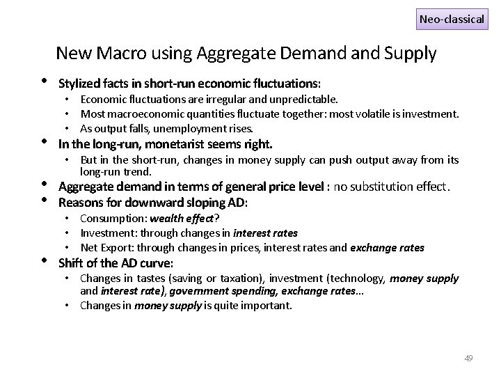
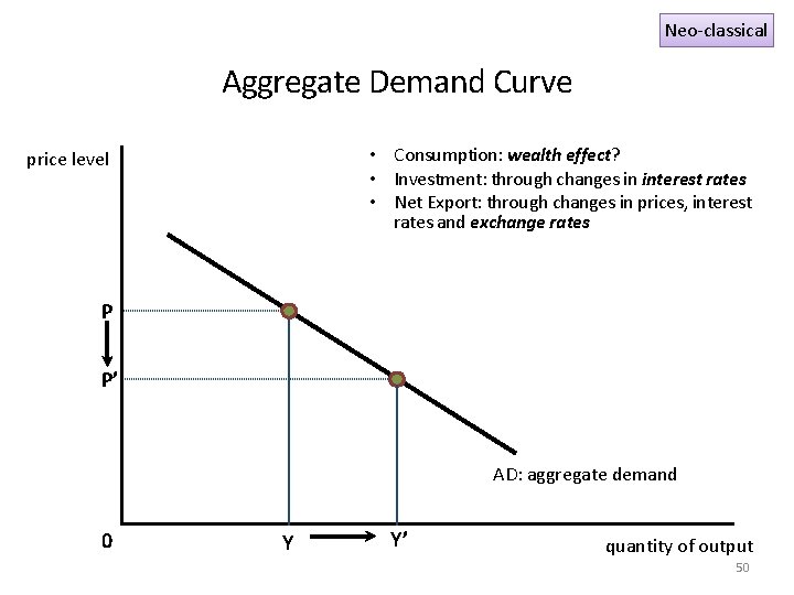
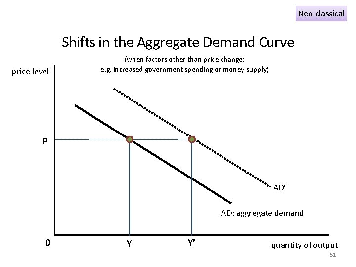
Neo-classical New Macro using Aggregate Demand Supply • Stylized facts in short-run economic fluctuations: • In the long-run, monetarist seems right. • • Aggregate demand in terms of general price level : no substitution effect. Reasons for downward sloping AD: • Shift of the AD curve: • Economic fluctuations are irregular and unpredictable. • Most macroeconomic quantities fluctuate together: most volatile is investment. • As output falls, unemployment rises. • But in the short-run, changes in money supply can push output away from its long-run trend. • Consumption: wealth effect? • Investment: through changes in interest rates • Net Export: through changes in prices, interest rates and exchange rates • Changes in tastes (saving or taxation), investment (technology, money supply and interest rate), government spending, exchange rates… • Changes in money supply is quite important. 49

Neo-classical Aggregate Demand Curve • Consumption: wealth effect? • Investment: through changes in interest rates • Net Export: through changes in prices, interest rates and exchange rates price level P P’ AD: aggregate demand 0 Y Y’ quantity of output 50

Neo-classical Shifts in the Aggregate Demand Curve price level (when factors other than price change; e. g. increased government spending or money supply) P AD’ AD: aggregate demand 0 Y Y’ quantity of output 51

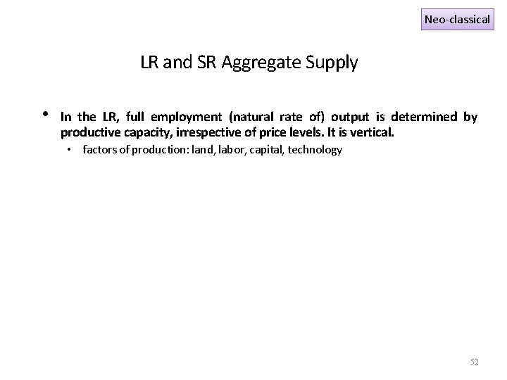
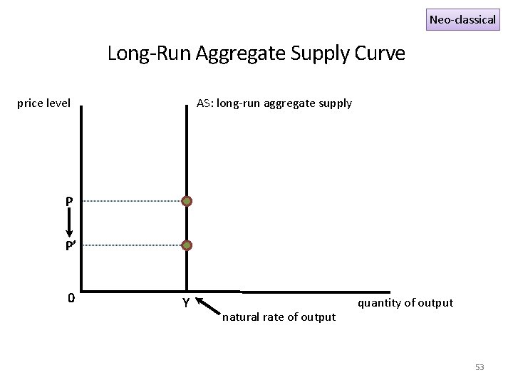
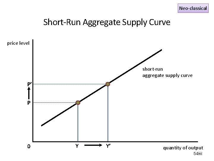
Neo-classical LR and SR Aggregate Supply • In the LR, full employment (natural rate of) output is determined by productive capacity, irrespective of price levels. It is vertical. • factors of production: land, labor, capital, technology 52

Neo-classical Long-Run Aggregate Supply Curve price level AS: long-run aggregate supply P P’ 0 Y natural rate of output quantity of output 53

Neo-classical Short-Run Aggregate Supply Curve price level short-run aggregate supply curve P’ P 0 Y Y’ quantity of output 54

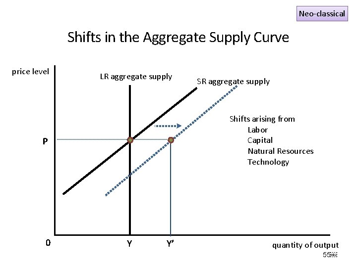
Neo-classical Shifts in the Aggregate Supply Curve price level LR aggregate supply Shifts arising from Labor Capital Natural Resources Technology P 0 SR aggregate supply Y Y’ quantity of output 55

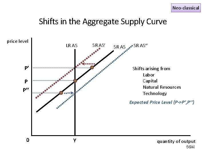
Neo-classical Shifts in the Aggregate Supply Curve price level LR AS P’ SR AS’’ Shifts arising from Labor Capital Natural Resources Technology P P’’ Expected Price Level (P->P’, P’’) 0 Y quantity of output 56

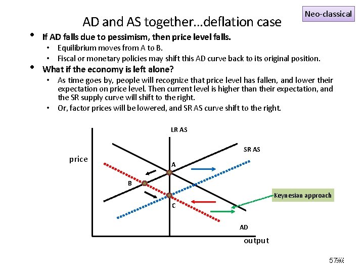
AD and AS together…deflation case • If AD falls due to pessimism, then price level falls. • What if the economy is left alone? Neo-classical • Equilibrium moves from A to B. • Fiscal or monetary policies may shift this AD curve back to its original position. • As time goes by, people will recognize that price level has fallen, and lower their expectation on price level. Then current level is higher than their expectation, and the SR supply curve will shift to the right. • Or, factor prices will be lowered, and SR AS curve shift to the right. LR AS SR AS price A B Keynesian approach C AD output 57

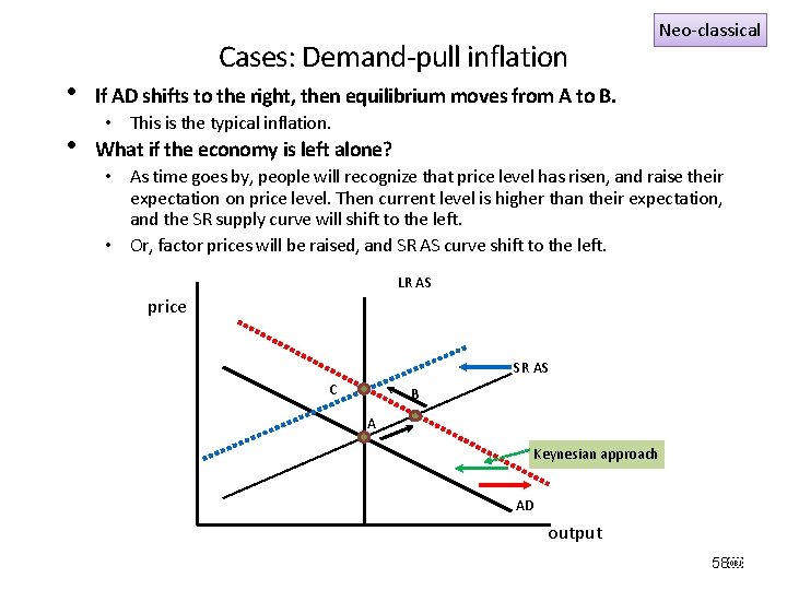
• • Cases: Demand-pull inflation Neo-classical If AD shifts to the right, then equilibrium moves from A to B. • This is the typical inflation. What if the economy is left alone? • As time goes by, people will recognize that price level has risen, and raise their expectation on price level. Then current level is higher than their expectation, and the SR supply curve will shift to the left. • Or, factor prices will be raised, and SR AS curve shift to the left. LR AS price SR AS C B A Keynesian approach AD output 58

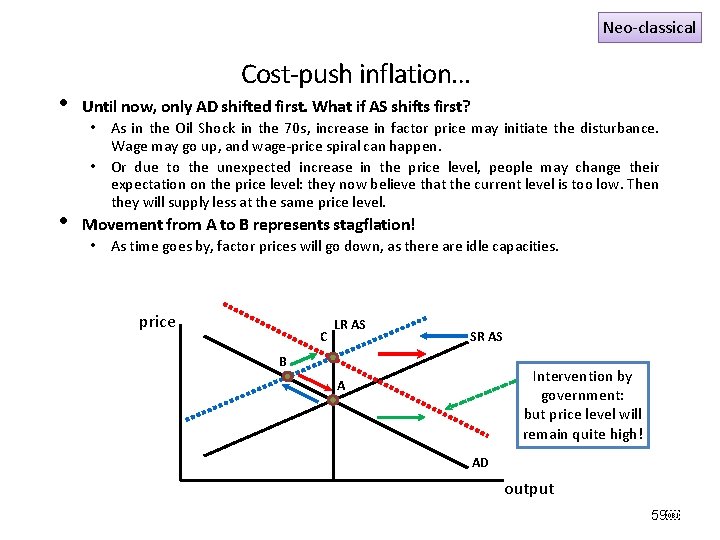
Neo-classical Cost-push inflation… • Until now, only AD shifted first. What if AS shifts first? • Movement from A to B represents stagflation! • As in the Oil Shock in the 70 s, increase in factor price may initiate the disturbance. Wage may go up, and wage-price spiral can happen. • Or due to the unexpected increase in the price level, people may change their expectation on the price level: they now believe that the current level is too low. Then they will supply less at the same price level. • As time goes by, factor prices will go down, as there are idle capacities. price C LR AS SR AS B Intervention by government: but price level will remain quite high! A AD output 59

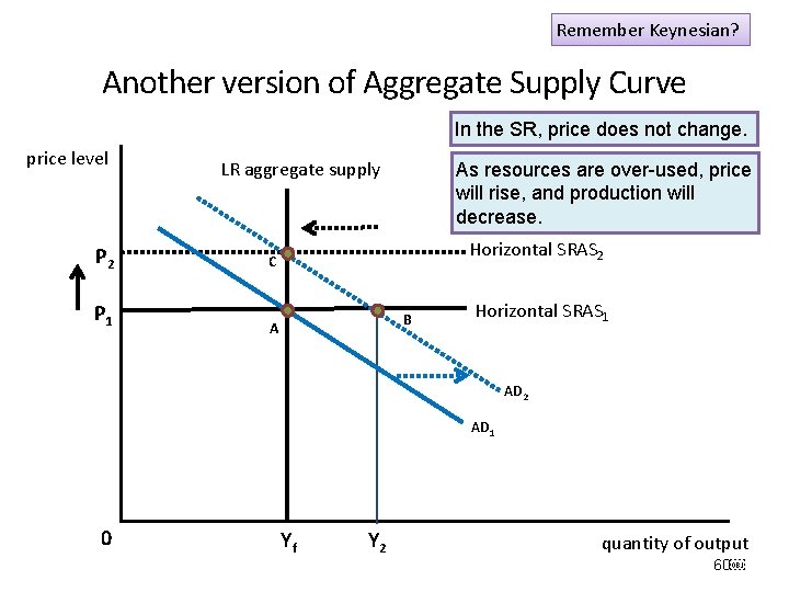
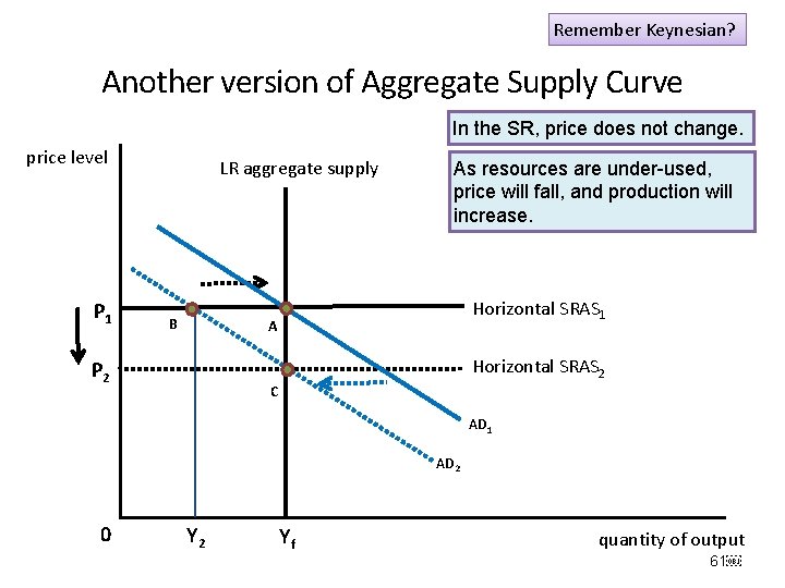
Remember Keynesian? Another version of Aggregate Supply Curve In the SR, price does not change. price level P 2 P 1 LR aggregate supply As resources are over-used, price will rise, and production will decrease. Horizontal SRAS 2 C B A Horizontal SRAS 1 AD 2 AD 1 0 Yf Y 2 quantity of output 60

Remember Keynesian? Another version of Aggregate Supply Curve In the SR, price does not change. price level P 1 LR aggregate supply B As resources are under-used, price will fall, and production will increase. Horizontal SRAS 1 A Horizontal SRAS 2 P 2 C AD 1 AD 2 0 Y 2 Yf quantity of output 61

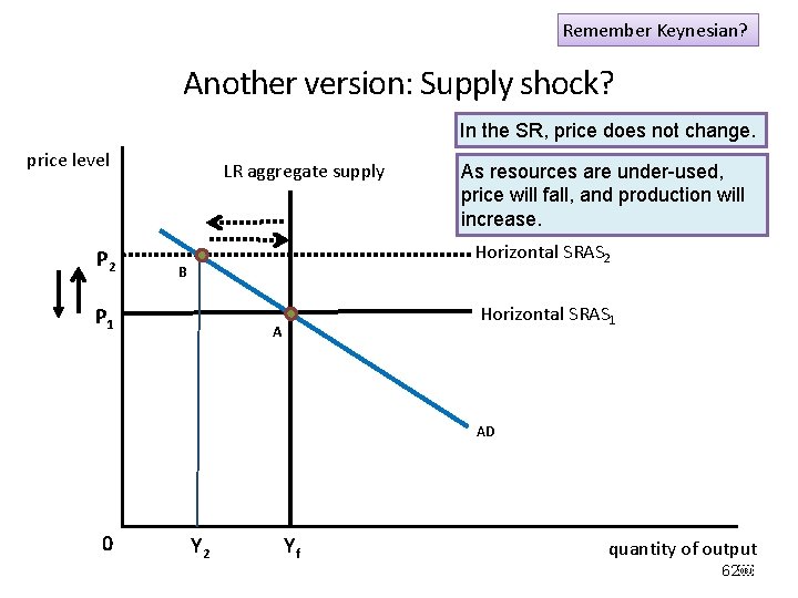
Remember Keynesian? Another version: Supply shock? In the SR, price does not change. price level P 2 LR aggregate supply As resources are under-used, price will fall, and production will increase. Horizontal SRAS 2 B P 1 Horizontal SRAS 1 A AD 0 Y 2 Yf quantity of output 62

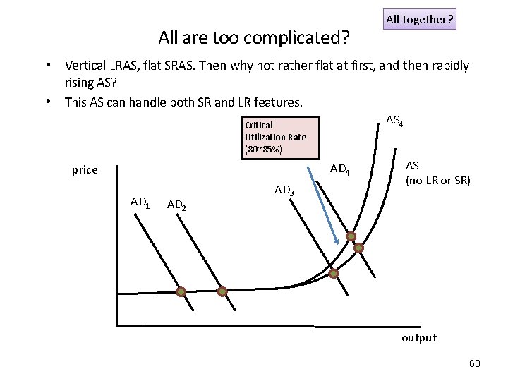
All are too complicated? All together? • Vertical LRAS, flat SRAS. Then why not rather flat at first, and then rapidly rising AS? • This AS can handle both SR and LR features. AS 4 Critical Utilization Rate (80~85%) AD 4 price AD 1 AD 2 AD 3 AS (no LR or SR) output 63

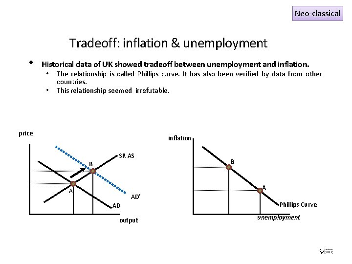
Neo-classical Tradeoff: inflation & unemployment • Historical data of UK showed tradeoff between unemployment and inflation. • • The relationship is called Phillips curve. It has also been verified by data from other countries. This relationship seemed irrefutable. price inflation B SR AS B A A AD’ AD output Phillips Curve unemployment 64

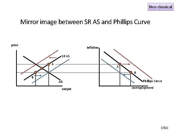
Neo-classical Mirror image between SR AS and Phillips Curve price inflation SR AS A A B B AD output Phillips Curve unemployment 65

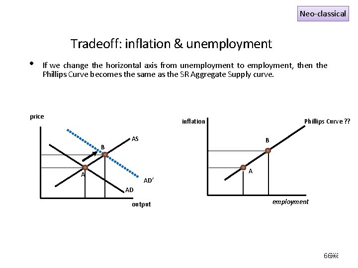
Neo-classical Tradeoff: inflation & unemployment • If we change the horizontal axis from unemployment to employment, then the Phillips Curve becomes the same as the SR Aggregate Supply curve. price Phillips Curve ? ? inflation B AS B A A AD’ AD output employment 66

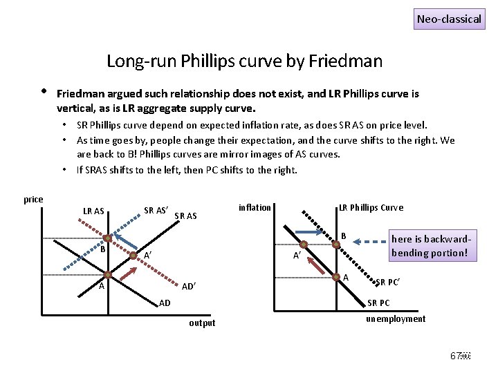
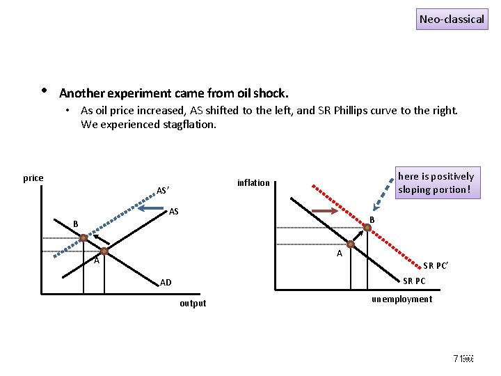
Neo-classical Long-run Phillips curve by Friedman • Friedman argued such relationship does not exist, and LR Phillips curve is vertical, as is LR aggregate supply curve. • SR Phillips curve depend on expected inflation rate, as does SR AS on price level. • As time goes by, people change their expectation, and the curve shifts to the right. We are back to B! Phillips curves are mirror images of AS curves. • If SRAS shifts to the left, then PC shifts to the right. price LR AS SR AS’ SR AS inflation LR Phillips Curve B B A’ here is backwardbending portion! A’ A AD’ A SR PC’ SR PC AD output unemployment 67

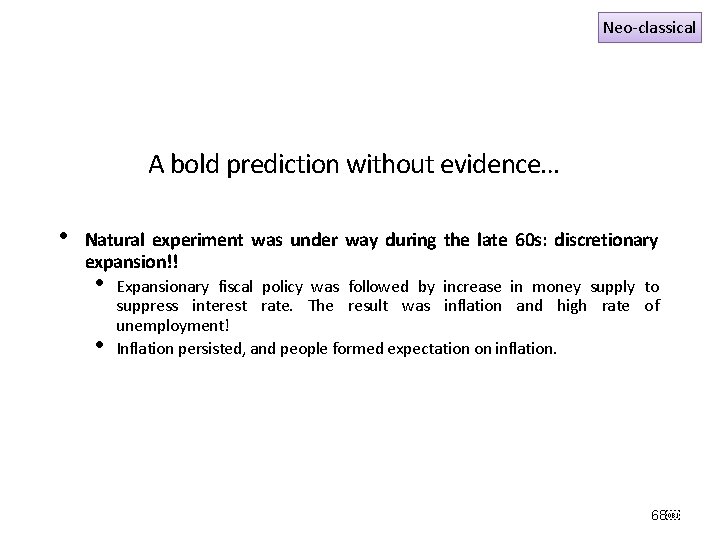
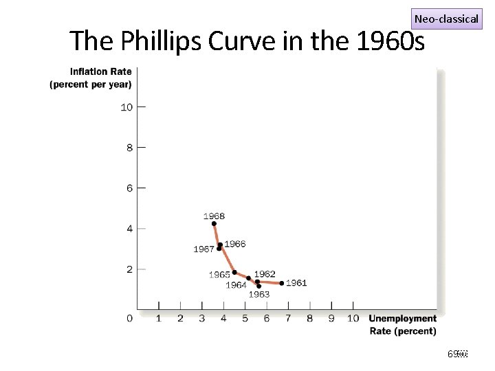
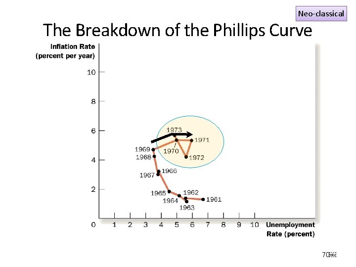
Neo-classical A bold prediction without evidence… • Natural experiment was under way during the late 60 s: discretionary expansion!! • • Expansionary fiscal policy was followed by increase in money supply to suppress interest rate. The result was inflation and high rate of unemployment! Inflation persisted, and people formed expectation on inflation. 68

Neo-classical The Phillips Curve in the 1960 s 69

Neo-classical The Breakdown of the Phillips Curve 70

Neo-classical • Another experiment came from oil shock. • As oil price increased, AS shifted to the left, and SR Phillips curve to the right. We experienced stagflation. price here is positively sloping portion! inflation AS’ AS B B A A SR PC’ SR PC AD output unemployment 71

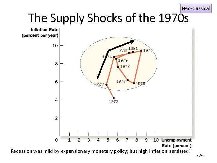
Neo-classical The Supply Shocks of the 1970 s Recession was mild by expansionary monetary policy; but high inflation persisted! 72

Neo-classical Sacrifice ratio and Rational Expectation • How quickly does expectation change to new monetary policy? • Sacrifice ratio: % in output decrease to decrease inflation by 1%. • If the ratio is 5, then 6% reduction in inflation required 30% decrease in output. 73

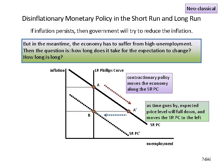
Neo-classical Disinflationary Monetary Policy in the Short Run and Long Run If inflation persists, then government will try to reduce the inflation. But in the meantime, the economy has to suffer from high-unemployment. Then the question is: how long does it take for the expectation to change? How long is long? inflation LR Phillips Curve A contractionary policy moves the economy along the SR PC A’ B as time goes by, expected price level will fall down, and moves the SR PC to the left SR PC’ unemployment 74

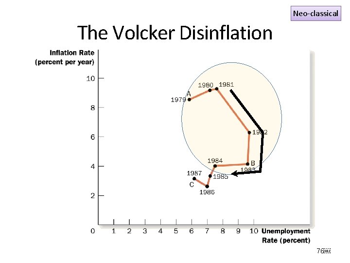
Neo-classical Sacrifice ratio and Rational Expectation • Emergence of Rational Expectations Theory • People adjust quickly, and sacrifice ratio would be rather small. It could even be zero. What is most important is the credibility of the policy. • Volcker disinflation took several years of deep recession. • But the cost was not as large as many economists claimed. Volcker’s tough stand might have had some direct effect on expectations. • Still many did not believe him, and expectation did not change as quickly. • No definite conclusion on Rational Expectations Theory, yet. 75

Neo-classical The Volcker Disinflation 76

Thanks a lot for your attention !! 77