ECE 700 07 Game Theory with Engineering Applications

ECE 700. 07: Game Theory with Engineering Applications Lecture 4: Computing Solution Concepts of Normal Form Games Seyed Majid Zahedi

Outline • Brief overview of (mixed integer) linear programs • Solving for • • Dominated strategies Minimax and maximin strategies Nash equilibrium Correlated NE • Readings: • MAS Appendix B, and Sec. 4

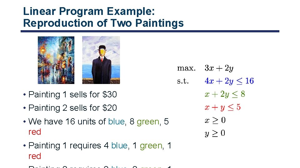
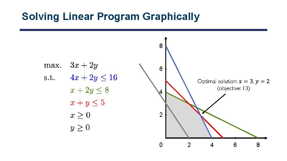
Linear Program Example: Reproduction of Two Paintings • Painting 1 sells for $30 • Painting 2 sells for $20 • We have 16 units of blue, 8 green, 5 red • Painting 1 requires 4 blue, 1 green, 1 red

Solving Linear Program Graphically 8 6 4 2 0 2 4 6 8

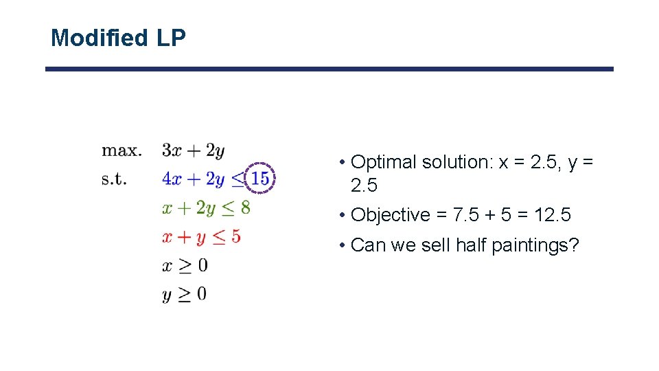
Modified LP • Optimal solution: x = 2. 5, y = 2. 5 • Objective = 7. 5 + 5 = 12. 5 • Can we sell half paintings?

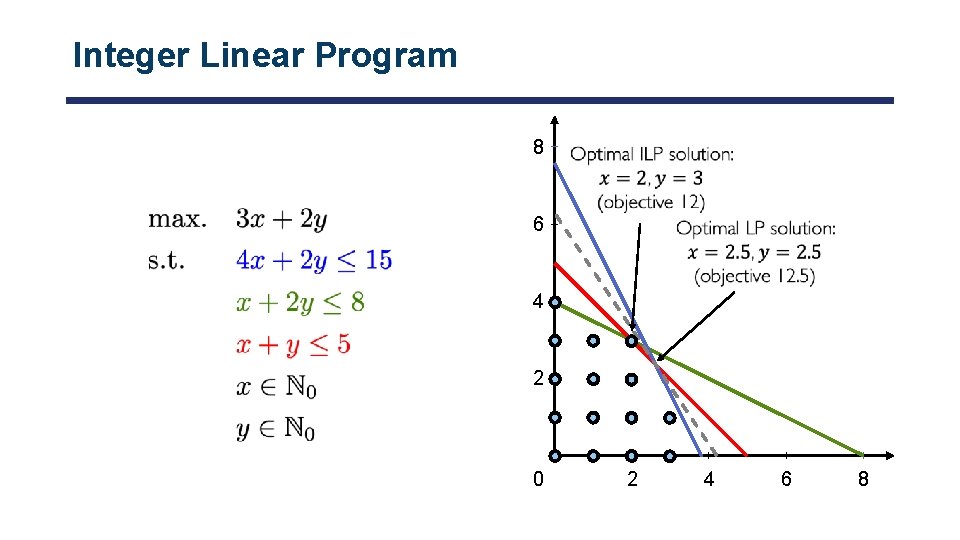
Integer Linear Program 8 6 4 2 0 2 4 6 8

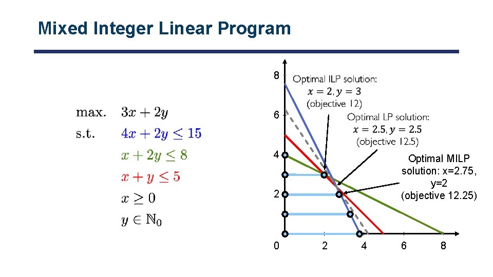
Mixed Integer Linear Program 8 6 4 Optimal MILP solution: x=2. 75, y=2 (objective 12. 25) 2 0 2 4 6 8

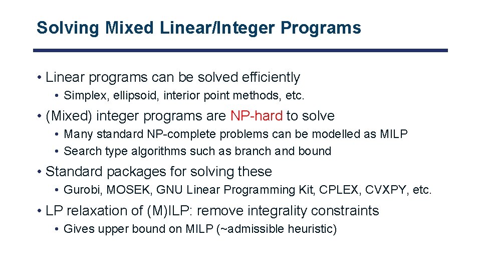
Solving Mixed Linear/Integer Programs • Linear programs can be solved efficiently • Simplex, ellipsoid, interior point methods, etc. • (Mixed) integer programs are NP-hard to solve • Many standard NP-complete problems can be modelled as MILP • Search type algorithms such as branch and bound • Standard packages for solving these • Gurobi, MOSEK, GNU Linear Programming Kit, CPLEX, CVXPY, etc. • LP relaxation of (M)ILP: remove integrality constraints • Gives upper bound on MILP (~admissible heuristic)

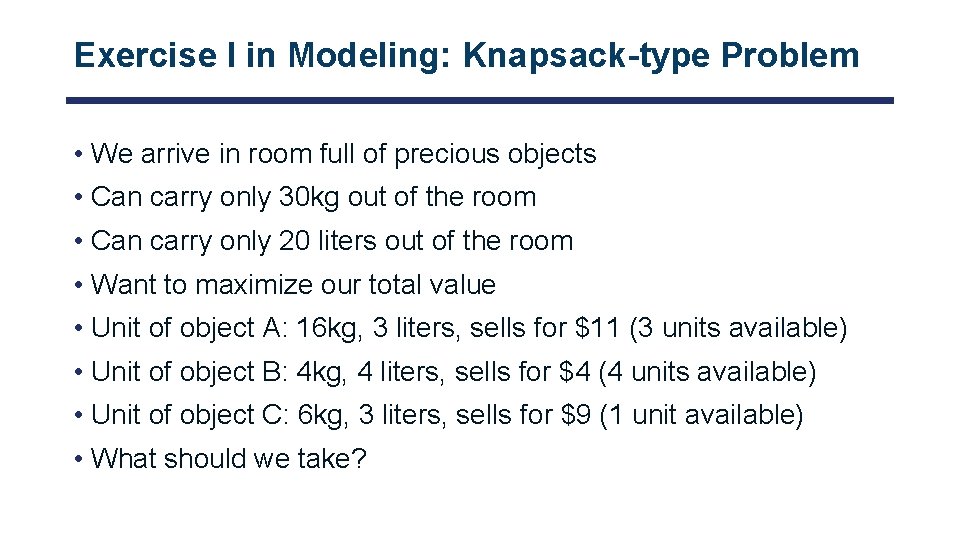
Exercise I in Modeling: Knapsack-type Problem • We arrive in room full of precious objects • Can carry only 30 kg out of the room • Can carry only 20 liters out of the room • Want to maximize our total value • Unit of object A: 16 kg, 3 liters, sells for $11 (3 units available) • Unit of object B: 4 kg, 4 liters, sells for $4 (4 units available) • Unit of object C: 6 kg, 3 liters, sells for $9 (1 unit available) • What should we take?

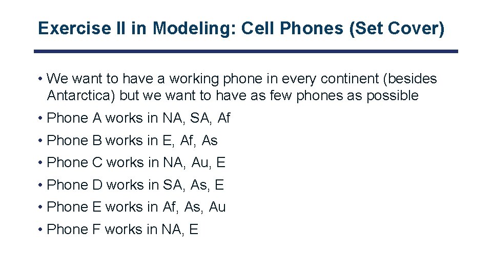
Exercise II in Modeling: Cell Phones (Set Cover) • We want to have a working phone in every continent (besides Antarctica) but we want to have as few phones as possible • Phone A works in NA, SA, Af • Phone B works in E, Af, As • Phone C works in NA, Au, E • Phone D works in SA, As, E • Phone E works in Af, As, Au • Phone F works in NA, E

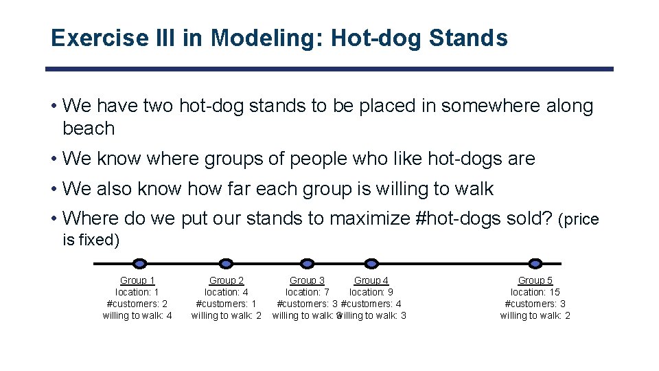
Exercise III in Modeling: Hot-dog Stands • We have two hot-dog stands to be placed in somewhere along beach • We know where groups of people who like hot-dogs are • We also know how far each group is willing to walk • Where do we put our stands to maximize #hot-dogs sold? (price is fixed) Group 1 location: 1 #customers: 2 willing to walk: 4 Group 2 location: 4 #customers: 1 willing to walk: 2 Group 3 Group 4 location: 7 location: 9 #customers: 3 #customers: 4 willing to walk: 3 Group 5 location: 15 #customers: 3 willing to walk: 2

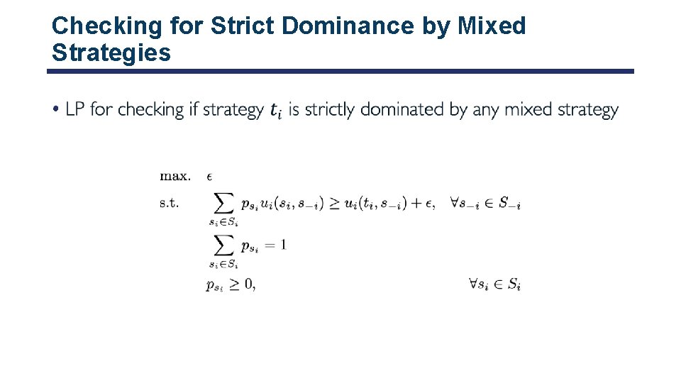
Checking for Strict Dominance by Mixed Strategies •

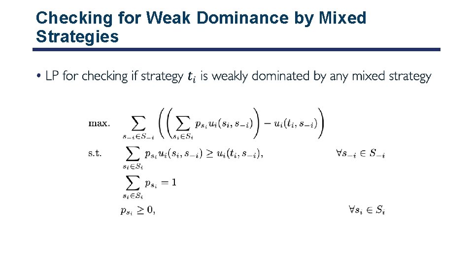
Checking for Weak Dominance by Mixed Strategies •

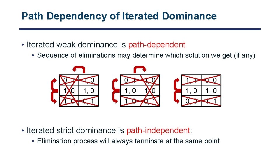
Path Dependency of Iterated Dominance • Iterated weak dominance is path-dependent • Sequence of eliminations may determine which solution we get (if any) 0, 1 1, 0 1, 0 0, 1 1, 0 0, 0 1, 1 • Iterated strict dominance is path-independent: • Elimination process will always terminate at the same point

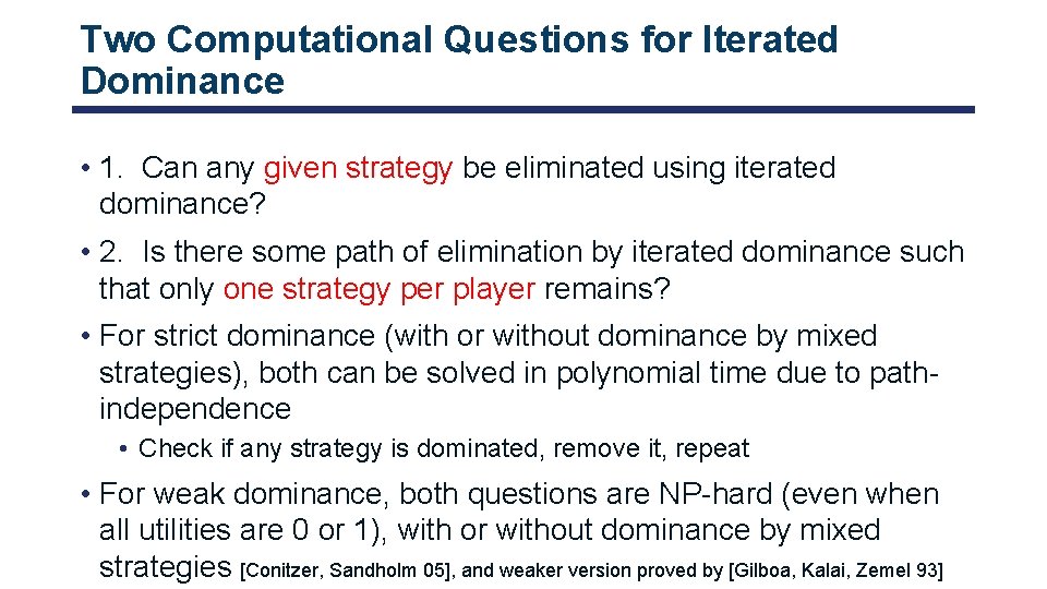
Two Computational Questions for Iterated Dominance • 1. Can any given strategy be eliminated using iterated dominance? • 2. Is there some path of elimination by iterated dominance such that only one strategy per player remains? • For strict dominance (with or without dominance by mixed strategies), both can be solved in polynomial time due to pathindependence • Check if any strategy is dominated, remove it, repeat • For weak dominance, both questions are NP-hard (even when all utilities are 0 or 1), with or without dominance by mixed strategies [Conitzer, Sandholm 05], and weaker version proved by [Gilboa, Kalai, Zemel 93]

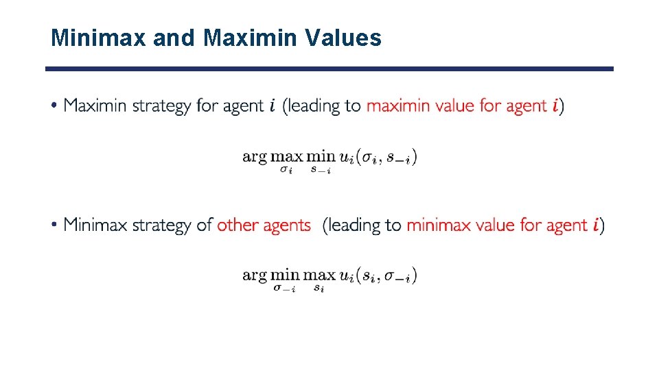
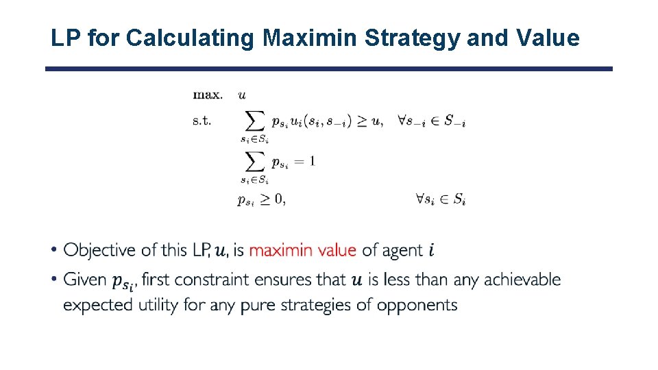
Minimax and Maximin Values •

LP for Calculating Maximin Strategy and Value •

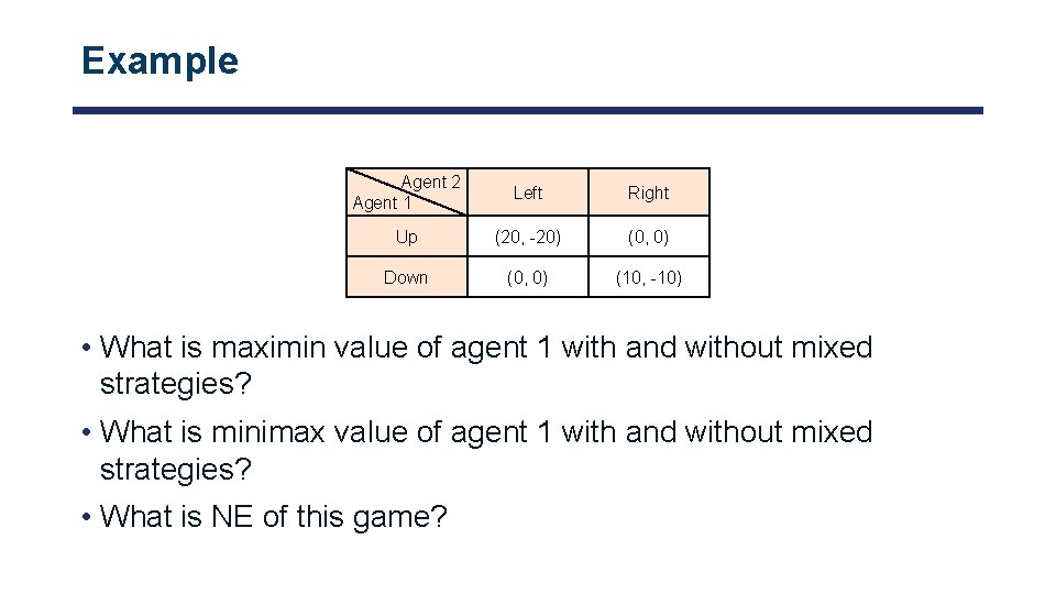
Minimax Theorem [von Neumann 1928] • Each player’s NE utility in any finite, two-player, zero-sum game is equal to her maximin value and minimax value • Minimax theorem does not hold with pure strategies only (example? )

Example Agent 2 Agent 1 Left Right Up (20, -20) (0, 0) Down (0, 0) (10, -10) • What is maximin value of agent 1 with and without mixed strategies? • What is minimax value of agent 1 with and without mixed strategies? • What is NE of this game?

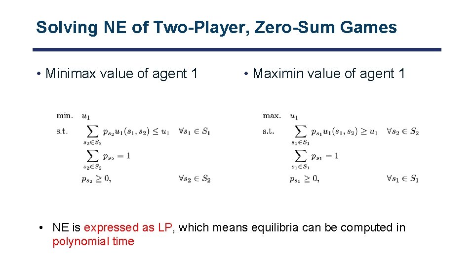
Solving NE of Two-Player, Zero-Sum Games • Minimax value of agent 1 • Maximin value of agent 1 • NE is expressed as LP, which means equilibria can be computed in polynomial time

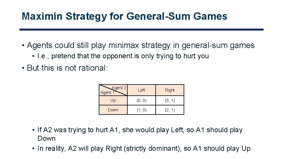
Maximin Strategy for General-Sum Games • Agents could still play minimax strategy in general-sum games • I. e. , pretend that the opponent is only trying to hurt you • But this is not rational: Agent 2 Agent 1 Left Right Up (0, 0) (3, 1) Down (1, 0) (2, 1) • If A 2 was trying to hurt A 1, she would play Left, so A 1 should play Down • In reality, A 2 will play Right (strictly dominant), so A 1 should play Up

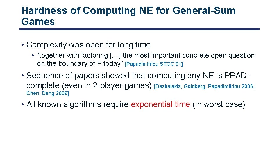
Hardness of Computing NE for General-Sum Games • Complexity was open for long time • “together with factoring […] the most important concrete open question on the boundary of P today” [Papadimitriou STOC’ 01] • Sequence of papers showed that computing any NE is PPADcomplete (even in 2 -player games) [Daskalakis, Goldberg, Papadimitriou 2006; Chen, Deng 2006] • All known algorithms require exponential time (in worst case)

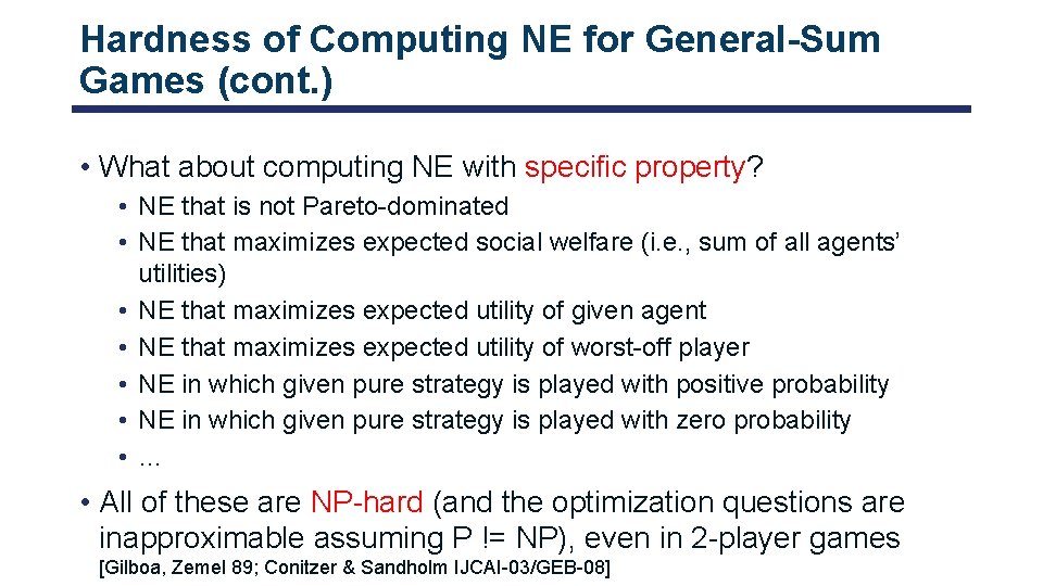
Hardness of Computing NE for General-Sum Games (cont. ) • What about computing NE with specific property? • NE that is not Pareto-dominated • NE that maximizes expected social welfare (i. e. , sum of all agents’ utilities) • NE that maximizes expected utility of given agent • NE that maximizes expected utility of worst-off player • NE in which given pure strategy is played with positive probability • NE in which given pure strategy is played with zero probability • … • All of these are NP-hard (and the optimization questions are inapproximable assuming P != NP), even in 2 -player games [Gilboa, Zemel 89; Conitzer & Sandholm IJCAI-03/GEB-08]

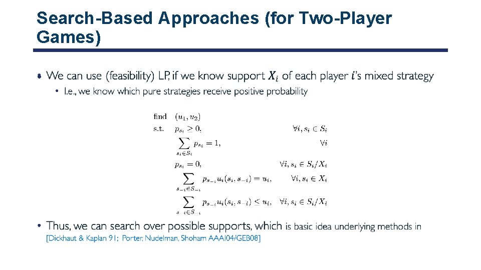
Search-Based Approaches (for Two-Player Games) •

Solving for NE using MILP (for Two-Player Games) [Sandholm, Gilpin, Conitzer AAAI 05] •

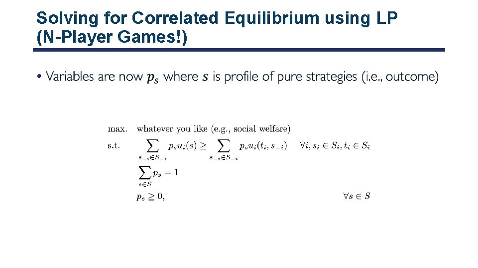
Solving for Correlated Equilibrium using LP (N-Player Games!) •

Questions?

Acknowledgement • This lecture is a slightly modified version of ones prepared by • Vincent Conitzer [Duke CPS 590. 4]