ECE 6382 Fall 2019 David R Jackson Notes

ECE 6382 Fall 2019 David R. Jackson Notes 6 Branch Points and Branch Cuts Notes are adapted from D. R. Wilton, Dept. of ECE 1

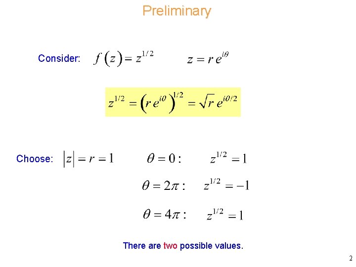
Preliminary Consider: Choose: There are two possible values. 2

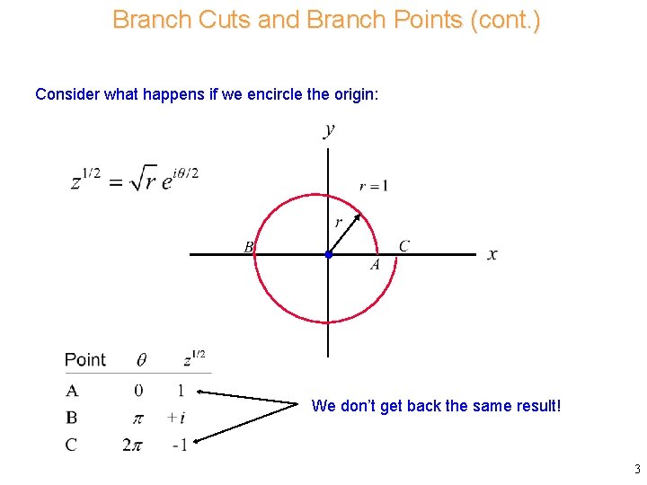
Branch Cuts and Branch Points (cont. ) Consider what happens if we encircle the origin: We don’t get back the same result! 3

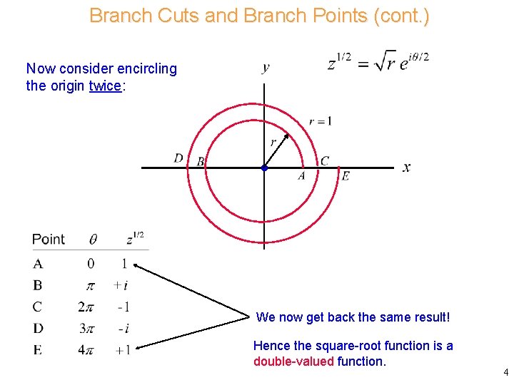
Branch Cuts and Branch Points (cont. ) Now consider encircling the origin twice: We now get back the same result! Hence the square-root function is a double-valued function. 4

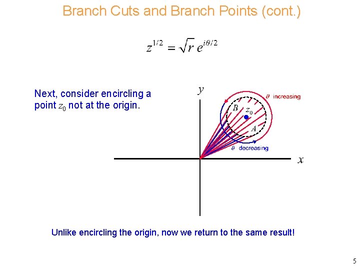
Branch Cuts and Branch Points (cont. ) Next, consider encircling a point z 0 not at the origin. Unlike encircling the origin, now we return to the same result! 5

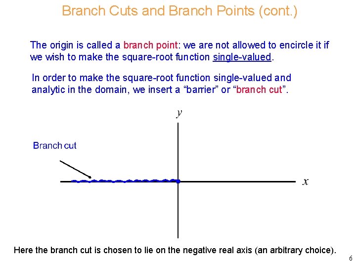
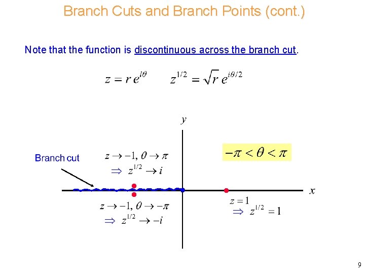
Branch Cuts and Branch Points (cont. ) The origin is called a branch point: we are not allowed to encircle it if we wish to make the square-root function single-valued. In order to make the square-root function single-valued analytic in the domain, we insert a “barrier” or “branch cut”. Here the branch cut is chosen to lie on the negative real axis (an arbitrary choice). 6

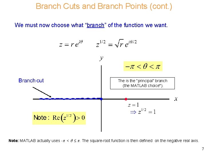
Branch Cuts and Branch Points (cont. ) We must now choose what “branch” of the function we want. The is the “principal” branch (the MATLAB choice*). Note: MATLAB actually uses - < . The square-root function is then defined on the negative real axis. 7

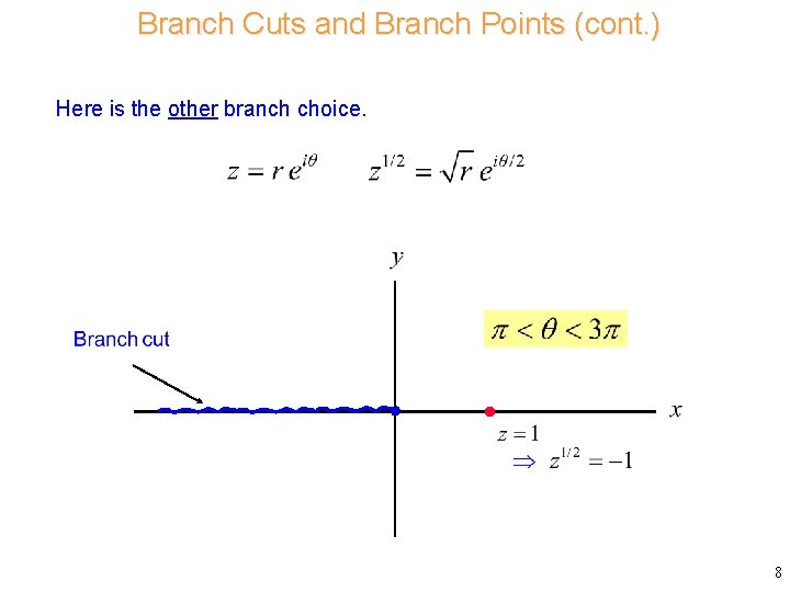
Branch Cuts and Branch Points (cont. ) Here is the other branch choice. 8

Branch Cuts and Branch Points (cont. ) Note that the function is discontinuous across the branch cut. 9

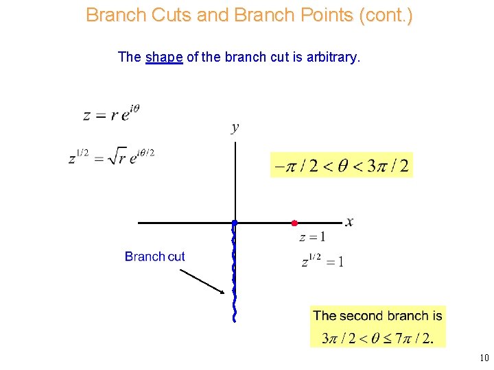
Branch Cuts and Branch Points (cont. ) The shape of the branch cut is arbitrary. 10

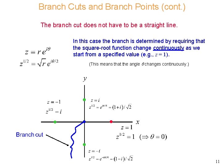
Branch Cuts and Branch Points (cont. ) The branch cut does not have to be a straight line. In this case the branch is determined by requiring that the square-root function change continuously as we start from a specified value (e. g. , z = 1). (This means that the angle changes continuously. ) 11

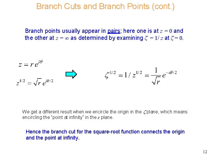
Branch Cuts and Branch Points (cont. ) Branch points usually appear in pairs; here one is at z = 0 and the other at z = ∞ as determined by examining ζ = 1/ z at ζ = 0. We get a different result when we encircle the origin in the plane, which means encircling the “point at infinity” in the z plane. Hence the branch cut for the square-root function connects the origin and the point at infinity. 12

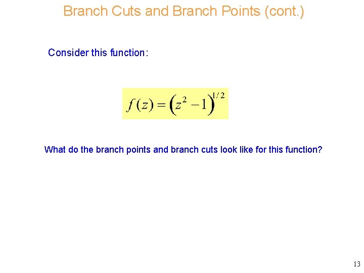
Branch Cuts and Branch Points (cont. ) Consider this function: What do the branch points and branch cuts look like for this function? 13

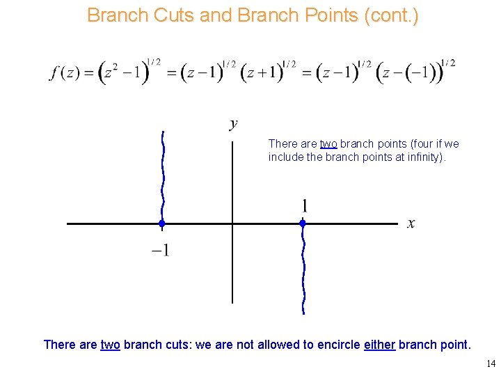
Branch Cuts and Branch Points (cont. ) There are two branch points (four if we include the branch points at infinity). There are two branch cuts: we are not allowed to encircle either branch point. 14

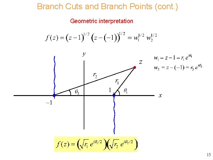
Branch Cuts and Branch Points (cont. ) Geometric interpretation 15

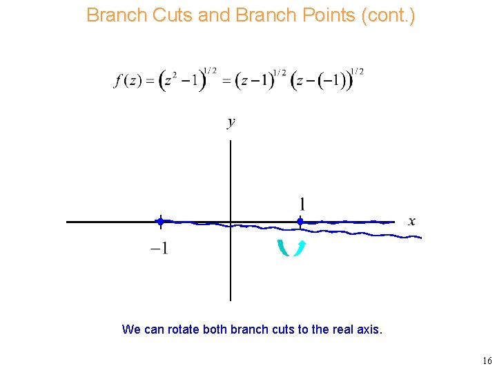
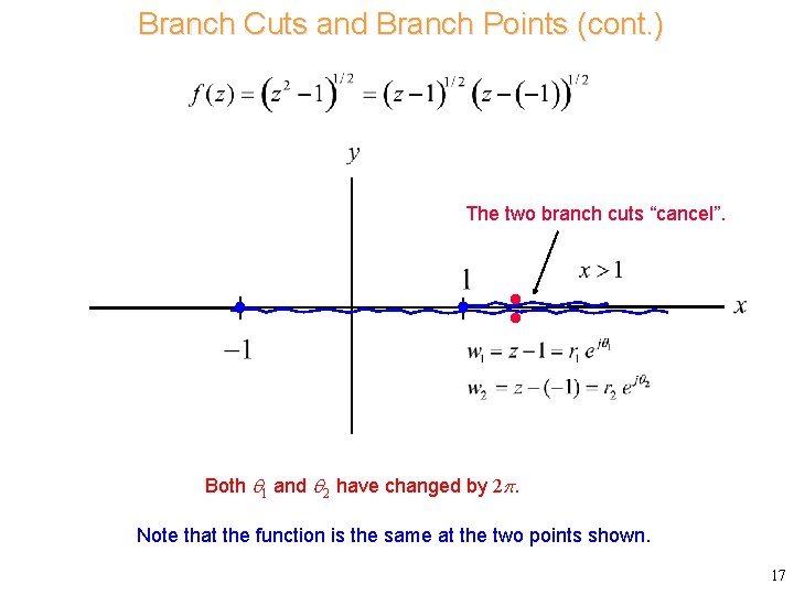
Branch Cuts and Branch Points (cont. ) We can rotate both branch cuts to the real axis. 16

Branch Cuts and Branch Points (cont. ) The two branch cuts “cancel”. Both 1 and 2 have changed by 2. Note that the function is the same at the two points shown. 17

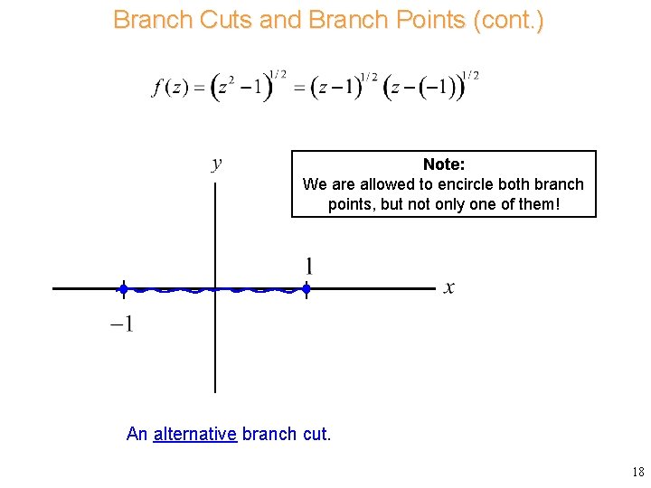
Branch Cuts and Branch Points (cont. ) Note: We are allowed to encircle both branch points, but not only one of them! An alternative branch cut. 18

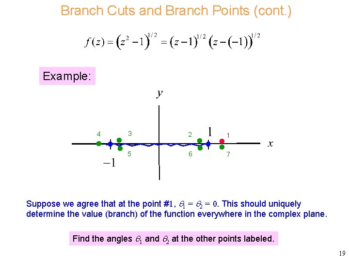
Branch Cuts and Branch Points (cont. ) Example: 4 3 2 1 5 6 7 Suppose we agree that at the point #1, 1 = 2 = 0. This should uniquely determine the value (branch) of the function everywhere in the complex plane. Find the angles 1 and 2 at the other points labeled. 19

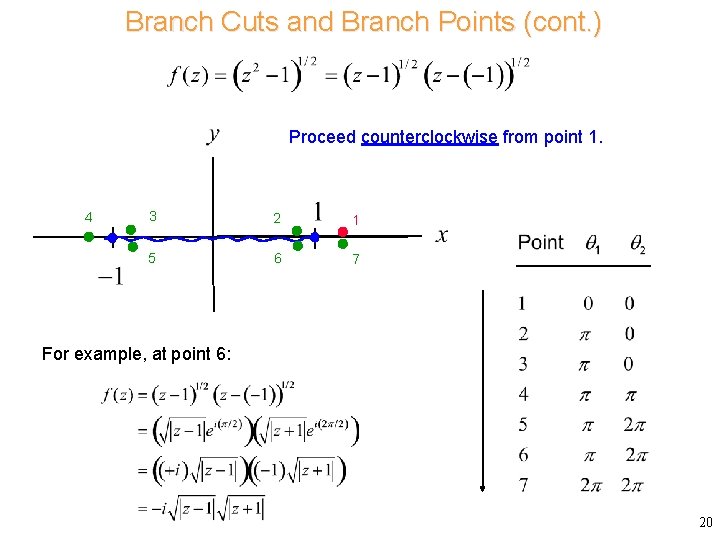
Branch Cuts and Branch Points (cont. ) Proceed counterclockwise from point 1. 4 3 2 1 5 6 7 For example, at point 6: 20

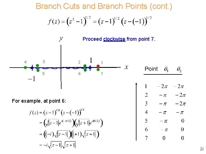
Branch Cuts and Branch Points (cont. ) Proceed clockwise from point 7. 4 3 2 1 5 6 7 For example, at point 6: 21

Sommerfeld Branch Cuts Arnold Sommerfeld (1868 -1951) Sommerfeld branch cuts are the most common choice in dealing with radiation types of problems, where there is a square-root wavenumber function. 22

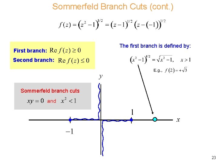
Sommerfeld Branch Cuts (cont. ) First branch: The first branch is defined by: Second branch: Sommerfeld branch cuts 23

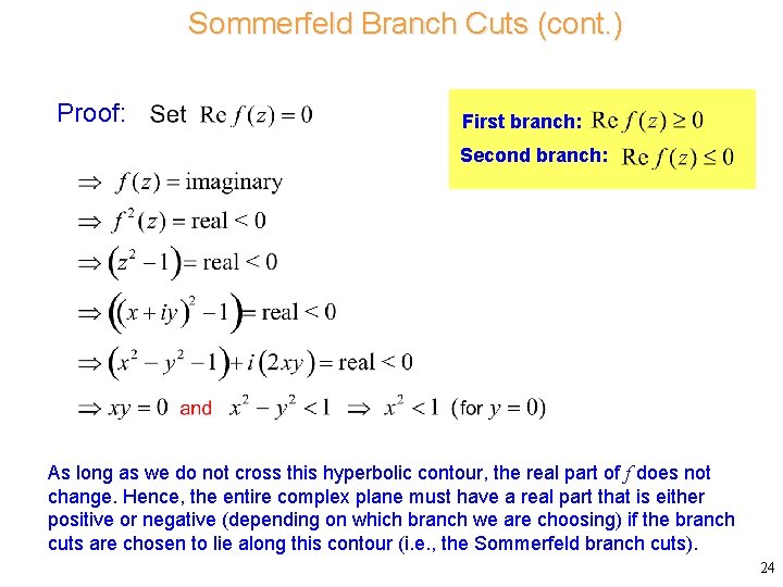
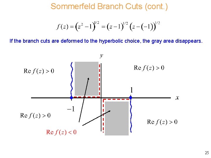
Sommerfeld Branch Cuts (cont. ) Proof: First branch: Second branch: As long as we do not cross this hyperbolic contour, the real part of f does not change. Hence, the entire complex plane must have a real part that is either positive or negative (depending on which branch we are choosing) if the branch cuts are chosen to lie along this contour (i. e. , the Sommerfeld branch cuts). 24

Sommerfeld Branch Cuts (cont. ) If the branch cuts are deformed to the hyperbolic choice, the gray area disappears. 25

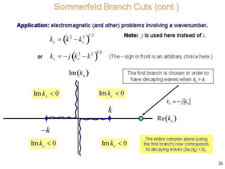
Sommerfeld Branch Cuts (cont. ) Application: electromagnetic (and other) problems involving a wavenumber. Note: j is used here instead of i. or (The – sign in front is an arbitrary choice here. ) The first branch is chosen in order to have decaying waves when kx > k. The entire complex plane (using the first branch) now corresponds to decaying waves (Im (kz) < 0). 26

Riemann Surface A Riemann surface is a surface that combines the different sheets of a multi-valued function. It is useful since it displays all possible values of the function at one time. (his signature) Georg Friedrich Bernhard Riemann (1826 -1866) 27

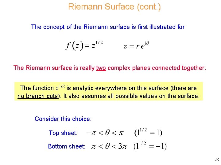
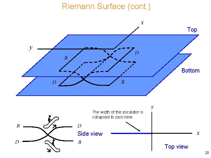
Riemann Surface (cont. ) The concept of the Riemann surface is first illustrated for The Riemann surface is really two complex planes connected together. The function z 1/2 is analytic everywhere on this surface (there are no branch cuts). It also assumes all possible values on the surface. Consider this choice: Top sheet: Bottom sheet: 28

Riemann Surface (cont. ) Top Bottom The width of the escalator is collapsed to zero here. Side view Top view 29

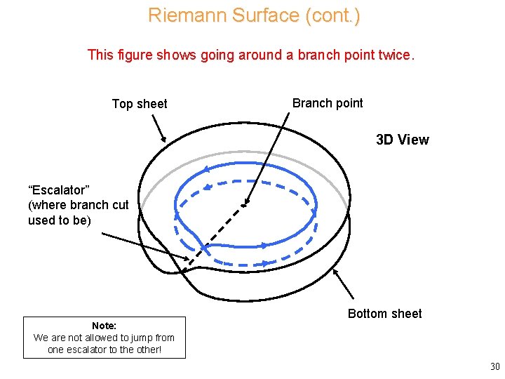
Riemann Surface (cont. ) This figure shows going around a branch point twice. Top sheet Branch point 3 D View “Escalator” (where branch cut used to be) Note: We are not allowed to jump from one escalator to the other! Bottom sheet 30

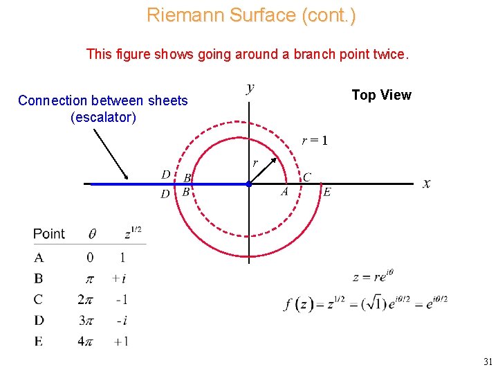
Riemann Surface (cont. ) This figure shows going around a branch point twice. Top View Connection between sheets (escalator) r=1 r 31

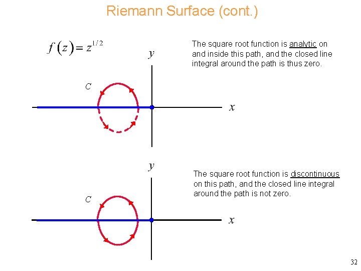
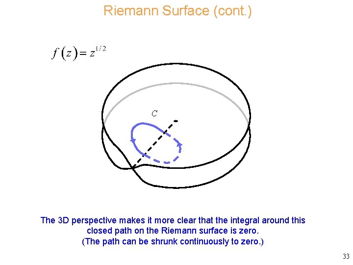
Riemann Surface (cont. ) The square root function is analytic on and inside this path, and the closed line integral around the path is thus zero. C C The square root function is discontinuous on this path, and the closed line integral around the path is not zero. 32

Riemann Surface (cont. ) C The 3 D perspective makes it more clear that the integral around this closed path on the Riemann surface is zero. (The path can be shrunk continuously to zero. ) 33

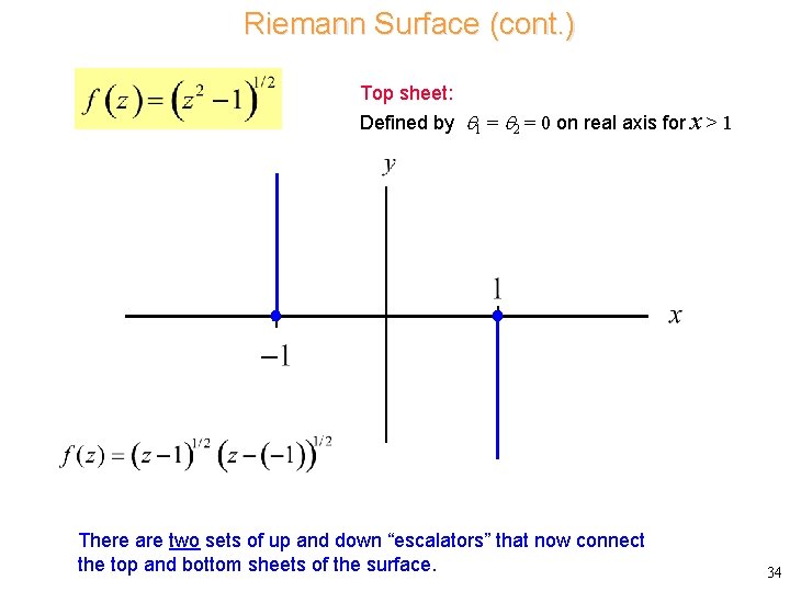
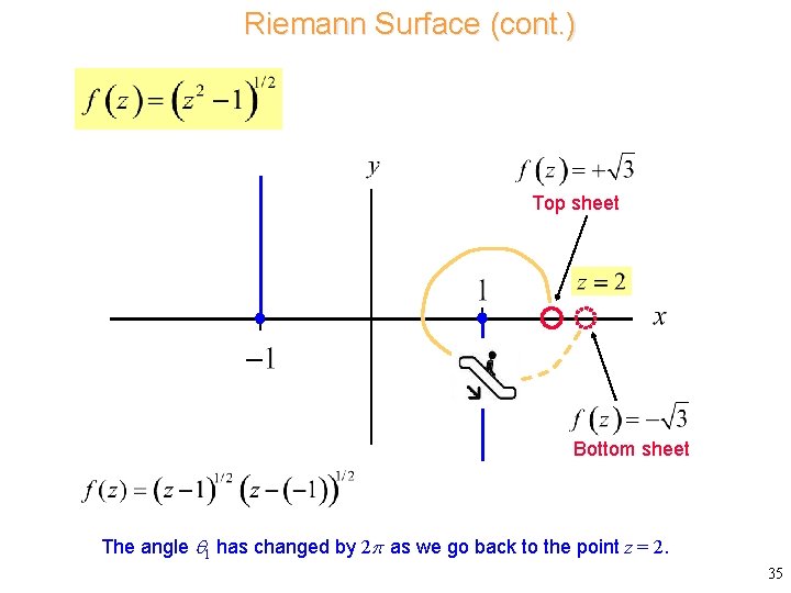
Riemann Surface (cont. ) Top sheet: Defined by 1 = 2 = 0 on real axis for x > 1 There are two sets of up and down “escalators” that now connect the top and bottom sheets of the surface. 34

Riemann Surface (cont. ) Top sheet Bottom sheet The angle 1 has changed by 2 as we go back to the point z = 2. 35

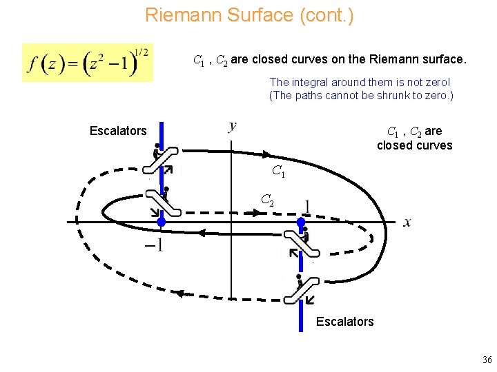
Riemann Surface (cont. ) C 1 , C 2 are closed curves on the Riemann surface. The integral around them is not zero! (The paths cannot be shrunk to zero. ) C 1 , C 2 are closed curves Escalators C 1 C 2 Escalators 36

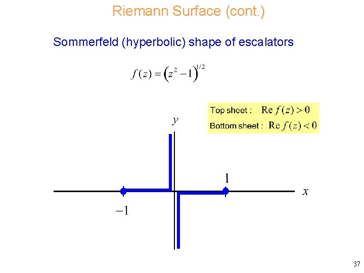
Riemann Surface (cont. ) Sommerfeld (hyperbolic) shape of escalators 37

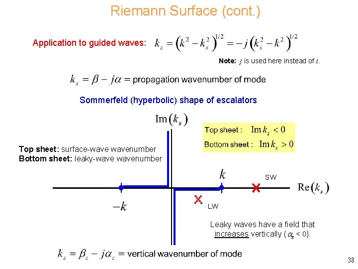
Riemann Surface (cont. ) Application to guided waves: Note: j is used here instead of i. Sommerfeld (hyperbolic) shape of escalators Top sheet: surface-wavenumber Bottom sheet: leaky-wavenumber SW LW Leaky waves have a field that increases vertically ( z < 0). 38

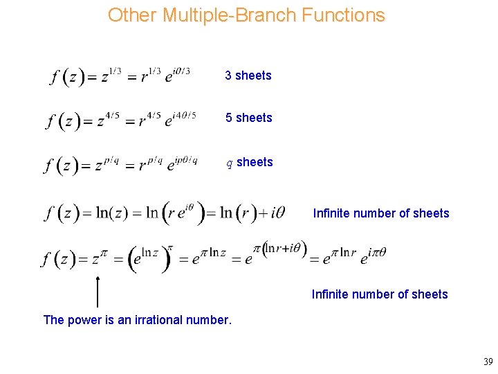
Other Multiple-Branch Functions 3 sheets 5 sheets q sheets Infinite number of sheets The power is an irrational number. 39

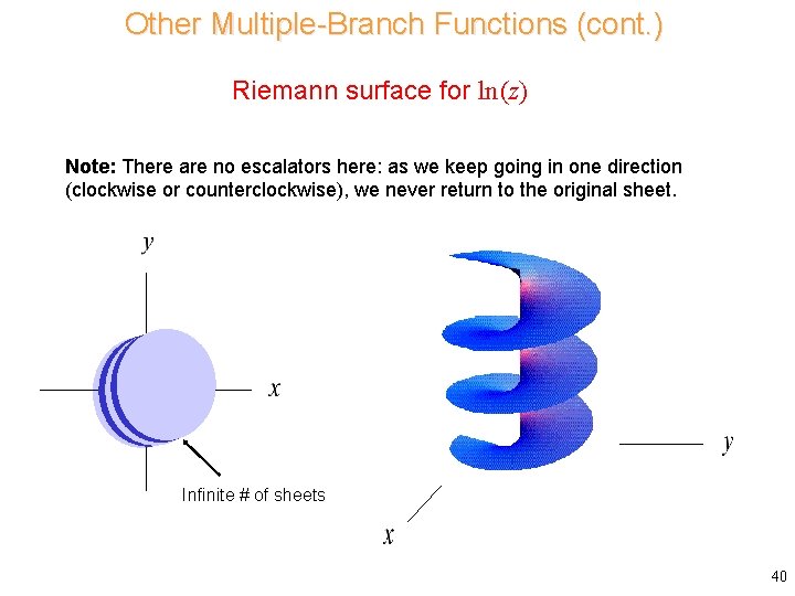
Other Multiple-Branch Functions (cont. ) Riemann surface for ln (z) Note: There are no escalators here: as we keep going in one direction (clockwise or counterclockwise), we never return to the original sheet. Infinite # of sheets 40