EAT 252 FLUID MECHANICS ENGINEERING CHAPTER 4 FLUID

EAT 252 FLUID MECHANICS ENGINEERING CHAPTER 4 FLUID DYNAMICS

Chapter Outline 1. Fluid Flow rate and the Continuity Equation 2. Conservation of Energy – Bernoulli’s Equation 3. Interpretation of Bernoulli’s Equation 4. Restrictions on Bernoulli’s Equation 5. Applications of Bernoulli’s Equation 6. Torricelli’s Theorem

4. 1 Fluid Flow Rate and the Continuity Equation The quantity of fluid flowing in a system per unit time can be expressed by the following three different terms: Q: (volume flow rate) is the volume of fluid flowing past a section per unit time. W (weight flow rate) is the weight of fluid flowing past a section per unit time. ṁ (mass flow rate) is the mass of fluid flowing past a section per unit time.

The most fundamental of these three terms is the volume flow rate Q, which is calculated from Q = Av (4 -1) where A is the area of the section and ν is the average velocity of flow. The units of Q can be derived as follows, using SI units for illustration: Q = Av = m 2 x m/s = m 3/s The weight flow rate W is related to Q by W = ϒQ (4 -2) where γ is the specific weight of the fluid. The units of W are then: W = ϒQ = N/m 3 x m 3/s = N/s

The mass flow rate ṁ is related to Q by: ṁ = ρQ The units of M are then ṁ = ρQ = kg/m 3 x m 3/s = kg/s Useful conversion given below: (4 -3)

Table 4. 2 shows the typical volume flow rates

Example 4. 1 Convert a flow rate of 30 gal/min to ft 3/s. The flow rate is

Example 4. 2 Convert a flow rate of 600 L/min to m 3/s.

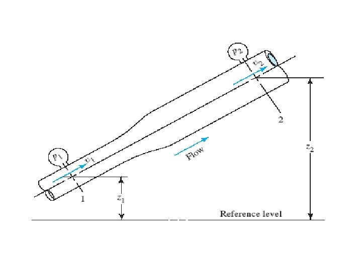
The method of calculating the velocity of flow of a fluid in a closed pipe system depends on the principle of continuity. Fig 4. 1 shows the portion of a fluid distribution system showing variations in velocity, pressure, and elevation. This can be expressed in terms of the mass flow rate as: ṁ1 = ṁ 2

As ṁ=ρAv, we have ρ 1 A 1 v 1 = ρ 2 A 2 v 2 (4. 4) Equation (4. 4) is a mathematical statement of the principle of continuity and is called the continuity equation. It is used to relate the fluid density, flow area, and velocity of flow at two sections of the system in which there is steady flow. It is valid for all fluids, whether gas or liquid.

If the fluid in the pipe in Fig. 4. 1 is a liquid that can be considered incompressible, then the terms ρ1 and ρ2 is the same. A 1 v 1 = A 2 v 2 (4. 5) Since Q = Av, Q 1 = Q 2 Equation (5. 5) is the continuity equation as applied to liquids; it states that for steady flow the volume flow rate is the same at any section.

Example 4. 3 In Fig. 4. 1 the inside diameters of the pipe at sections 1 and 2 are 50 mm and 100 mm, respectively. Water at is flowing with an average velocity of 8 m/s at section 1. Calculate the following: (a) Velocity at section 2 (b) Volume flow rate (c) Weight flow rate (d) Mass flow rate

Example 4. 3 (Answer) (a) Velocity at section 2. From Eq. (4. 5) we have

Example 4. 3 (Answer) Then the velocity at section 2 is Notice that for steady flow of a liquid, as the flow area increases, the velocity decreases. This is independent of pressure and elevation.

Example 4. 3 (Answer) (b) Volume flow rate Q. From Table 4. 1, Q = v. A. Because of the principle of continuity we could use the conditions either at section 1 or at section 2 to calculate Q. At section 1 we have

Example 4. 3 (Answer) (c) Weight flow rate W. From Table 4. 1, W = γQ. At 70°C, the specific weight of water is 9. 59 k. N/m 3. Then the weight flow rate is

Example 4. 3 (Answer) (d) Mass flow rate ṁ. From Table 4. 1, ṁ = ρQ. At the 70 °C, the density of water is 978 kg/m 3. Then, the mass flow rate is

Example 4. 4 At the one section of air distribution system, air at 101. 35 k. Pa and 40 °C has an average velocity of 6. 1 m/s and the duct is 30. 5 cm square. At the another section, the duct is round with a diameter of 457 mm, and the velocity is measured to be 4. 57 m/s. Calculate: a) The density of air in the round section. b) The weight flow rate of air in N/s Given, At 101. 35 k. Pa and 40 °C, the density of air is 1. 134 kg/m 3 and the specific weight is 11. 14 N/m 3.

Example 4. 4 (Answer) According to the continuity equation for gases, Eq. (4. 4), we have Then, we can calculate the area of the two sections and solve for ρ2

Example 4. 4 (Answer) (a) Then, the density of the air in the round section is (b) The weight flow rate can be found at section 1. Then, the weight flow rate is

4. 2 Conservation of Energy – Bernoulli’s Equation In physics you learned that energy can be neither created nor destroyed, but it can be transformed from one form into another. This is a statement of the law of conservation of energy. Fig 4. 3 shows the element of a fluid in a pipe.

There are three forms of energy that are always considered when analyzing a pipe flow problem. 1. Potential Energy. Due to its elevation, the potential energy of the element relative to some reference level is: PE = mgz = wz (4 -6) where w is the weight of the element. 2. Kinetic Energy. Due to its velocity, the kinetic energy of the element is: KE = mv 2/2 = wv 2/2 g (4. 7)

3. Flow Energy. Sometimes called pressure energy or flow work, this represents the amount of work necessary to move the element of fluid across a certain section against the pressure p. Flow energy is abbreviated FE and is calculated from: FE = wp/ϒ (4. 8) Equation (5. 8) can be derived as follows: The work done is: W = p. AL = p. V where V is the volume of the element. The weight of the element w is: w = ϒV where γ is the specific weight of the fluid. Then, the volume of the element is: V = w/ϒ

And we have Eq. (4 -8) Fig 4. 4 shows the flow energy. The total amount of energy of these three forms possessed by the element of fluid is the sum E,

Each of these terms is expressed in units of energy, which are Newton-meters (Nm) in the SI unit system and foot-pounds (ft-lb) in the U. S. Customary System. Fig 4. 5 shows the fluid elements used in Bernoulli’s equation.

At section 1 and 2, the total energy is If no energy is added to the fluid or lost between sections 1 and 2, then the principle of conservation of energy requires that

The weight of the element w is common to all terms and can be divided out. The equation then becomes (4. 9) This is referred to as Bernoulli’s equation.

Example 4. 5 Kerosene with a specific weight of 7. 855 k. N/m 3 is flowing at 37. 85 L/min from pipe with diameter of 25 mm to a pipe with a diameter of 50 mm. Calculate the difference in pressure between these 2 pipes. Given that, point 1 is 3. 5 m below the point 2.

Each term in Bernoulli’s equation, Eq. (5. 9), resulted from dividing an expression for energy by the weight of an element of the fluid. Each term in Bernoulli’s equation is one form of the energy possessed by the fluid per unit weight of fluid flowing in the system. The units for each term are “energy per unit weight. ” In the SI system the units are Nm/N and in the U. S. Customary System the units are lb. ft/lb.

Fig 4. 6 shows the pressure head, elevation head, velocity head, and total head.

4. 3 Interpretation of Bernoulli’s Equation In Fig. 4. 6 you can see that the velocity head at section 2 will be less than that at section 1. This can be shown by the continuity equation, In summary, Bernoulli’s equation accounts for the changes in elevation head, pressure head, and velocity head between two points in a fluid flow system. It is assumed that there are no energy losses or additions between the two points, so the total head remains constant.

4. 4 Restriction on Bernoulli’s Equation Although Bernoulli’s equation is applicable to a large number of practical problems, there are several limitations that must be understood to apply it properly. 1. It is valid only for incompressible fluids because the specific weight of the fluid is assumed to be the same at the two sections of interest. 2. There can be no mechanical devices between the two sections of interest that would add energy to or remove energy from the system, because the equation states that the total energy in the fluid is constant.

3. There can be no heat transferred into or out of the fluid. 4. There can be no energy lost due to friction. In reality no system satisfies all these restrictions. However, there are many systems for which only a negligible error will result when Bernoulli’s equation is used. Also, the use of this equation may allow a fast estimate of a result when that is all that is required.

Example 4. 6 In Fig. 4. 6, water at 10 °C is flowing from section 1 to section 2. At section 1, which is 25 mm in diameter, the gage pressure is 345 k. Pa and the velocity of flow is 3. 0 m/s. Section 2, which is 50 mm in diameter, is 2. 0 m above section 1. Assuming there are no energy losses in the system, calculate the pressure p 2. List the items that are known from the problem statement before looking at the next panel.

Example 4. 6 (Answer) The pressure p 2 is to be found. In other words, we are asked to calculate the pressure at section 2, which is different from the pressure at section 1 because there is a change in elevation and flow area between the two sections. We are going to use Bernoulli’s equation to solve the problem. Which two sections should be used when writing the equation?

Example 4. 6 (Answer) Now write Bernoulli’s equation. The three terms on the left refer to section 1 and the three on the right refer to section 2.

Example 4. 6 (Answer) The final solution for p 2 should be The continuity equation is used: This is found from

Example 4. 6 (Answer) Now substitute the known values into Eq. (4– 10). The details of the solution are The pressure p 2 is a gage pressure because it was computed relative to p 1, which was also a gage pressure. In later problem solutions, we will assume the pressures to be gage unless otherwise stated.

4. 5 Application of Bernoulli’s Theorem: Tanks, Reservoirs and Nozzles Exposed to the Atmosphere When the fluid at a reference point is exposed to the atmosphere, the pressure is zero and the pressure head term can be cancelled from Bernoulli’s equation. Fig 4. 7 shows the siphon.

The tank from which the fluid is being drawn can be assumed to be quite large compared to the size of the flow area inside the pipe. The velocity head at the surface of a tank or reservoir is considered to be zero and it can be cancelled from Bernoulli’s equation. When the two points of reference for Bernoulli’s equation are both inside a pipe of the same size, the velocity head terms on both sides of the equation are equal and can be cancelled. When the two points of reference for Bernoulli’s equation are both at the same elevation, the elevation head terms z 1 and z 2 are equal and can be cancelled.

Example 4. 7 Figure 4. 7 shows a siphon that is used to draw water from a swimming pool. The pipe that makes up the siphon has an inside diameter of 40 mm and terminates with a 25 -mm diameter nozzle. Assuming that there are no energy losses in the system, calculate the volume flow rate through the siphon and the pressure at points B –E.

Example 4. 7 (Answer) The first step in this problem solution is to calculate the volume flow rate Q, using Bernoulli’s equation. The two most convenient points to use for this calculation are A and F. What is known about point A? Point A is the free surface of the water in the pool. Therefore, p. A = 0 Pa. Also, because the surface area of the pool is very large, the velocity of the water at the surface is very nearly zero. Therefore, we will assume v. A = 0.

Point F is in the free stream of water outside the nozzle. Because the stream is exposed to atmospheric pressure, the pressure p. F = 0 Pa. We also know that point F is 3. 0 m below point A. Because p. A = 0 Pa, p. F = 0 Pa , and v. A is approximately zero, we cancel the from the equation. What remains is

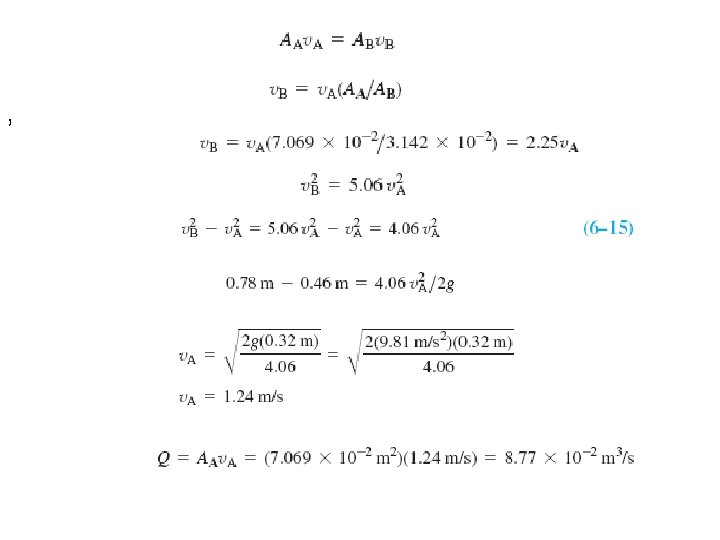
The objective is to calculate the volume flow rate, which depends on the velocity. The result is Using the continuing equation , compute the volume flow rate.

Points A and B are the best. As shown in the previous panels, using point A allows the equation to be simplified greatly, and because we are looking for p. B, we must choose point B. Write Bernoulli’s equation for points A and B, simplify it as before, and solve for p. B. Because p. A = 0 and v. A = 0, we have

We can calculate v. A by using the continuity equation:

The pressure at point B is The negative sign indicates that p. B is 4. 50 k. Pa below atmospheric pressure. Notice that when we deal with fluids in motion, the concept that points on the same level have the same pressure does not apply as it does with fluids at rest.

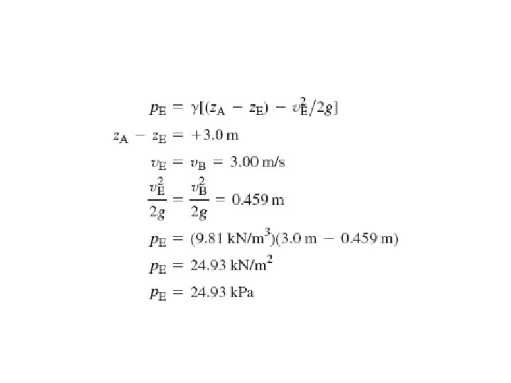
The next three panels present the solutions for the pressures p. C, p. D, and p. E, which can be found in a manner very similar to that used for p. B. Complete the solution for p. C before looking at the next panel. The answer is p. C = -16. 27 k. Pa. We use Bernoulli’s equation.

Because p. A = 0 and v. A = 0, the pressure at point C is

The pressure at point E is 24. 93 k. Pa. We use Bernoulli’s equation: Because p. A = 0 and v. A = 0, we have

5. 6 Application of Bernoulli’s Theorem: Venturi Meters & Other Closed Systems with Unknown Velocities Figure 4. 8 shows a device called a venturi meter that can be used to measure the velocity of flow in a fluid flow system.

The analysis of such a device is based on the application of Bernoulli’s equation. The reduced-diameter section at B causes the velocity of flow to increase there with a corresponding decrease in the pressure. It will be shown that the velocity of flow is dependent on the difference in pressure between points A and B. Therefore, a differential manometer as shown is convenient to use.

Example 4. 8 The venturi meter shown in Fig. 4. 8 carries water at 60°C. The specific gravity of the gage fluid in the manometer is 1. 25. Calculate the velocity of flow at section A and the volume flow rate of water.

Example 4. 8

4. 7 Torricelli’s Theorem Fig 4. 9 shows the flow from a tank.

Fluid is flowing from the side of a tank through a smooth, rounded nozzle. To determine the velocity of flow from the nozzle, write Bernoulli’s equation between a reference point on the fluid surface and a point in the jet issuing from the nozzle:

Example 4. 9 For the tank shown in Fig. 4. 9, compute the velocity of flow from the nozzle for a fluid depth h of 3. 00 m. Answer: This is a direct application of Torricelli’s theorem: