Detecting Anomalies in Space and Time with Application

Detecting Anomalies in Space and Time with Application to Biosurveillance Ronald D. Fricker, Jr. August 15, 2008

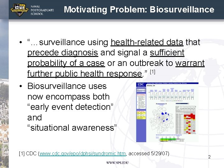
Motivating Problem: Biosurveillance • “…surveillance using health-related data that precede diagnosis and signal a sufficient probability of a case or an outbreak to warrant further public health response. ” [1] • Biosurveillance uses now encompass both “early event detection” and “situational awareness” [1] CDC (www. cdc. gov/epo/dphsi/syndromic. htm, accessed 5/29/07) 2

Definitions • Early event detection: gathering and analyzing data in advance of diagnostic case confirmation to give early warning of a possible outbreak • Situational awareness: the real-time analysis and display of health data to monitor the location, magnitude, and spread of an outbreak 3

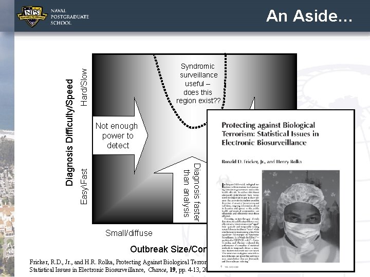
Hard/Slow Syndromic surveillance useful – does this region exist? ? Not enough power to detect Obvious – no fancy stats required EasyFast Diagnosis faster than analysis Diagnosis Difficulty/Speed An Aside… Small/diffuse Large/concentrated Outbreak Size/Concentration Fricker, R. D. , Jr. , and H. R. Rolka, Protecting Against Biological Terrorism: Statistical Issues in Electronic Biosurveillance, Chance, 19, pp. 4 -13, 2006. 4

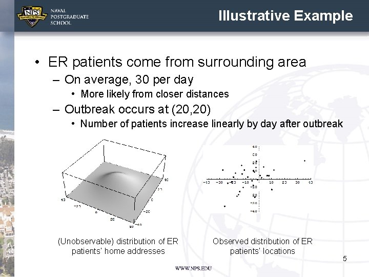
Illustrative Example • ER patients come from surrounding area – On average, 30 per day • More likely from closer distances – Outbreak occurs at (20, 20) • Number of patients increase linearly by day after outbreak (Unobservable) distribution of ER patients’ home addresses Observed distribution of ER patients’ locations 5

A Couple of Major Assumptions • Can geographically locate individuals in a medically meaningful way – Non-trivial problem – Data not currently available • Data is reported in a timely and consistent manner – Public health community working this problem, but not solved yet • Assuming the above problems away… 6

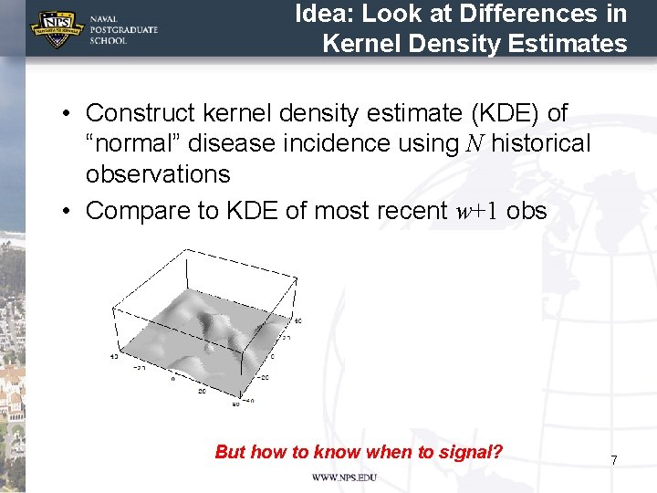
Idea: Look at Differences in Kernel Density Estimates • Construct kernel density estimate (KDE) of “normal” disease incidence using N historical observations • Compare to KDE of most recent w+1 obs But how to know when to signal? 7

Solution: Repeated Two-Sample Rank (RTR) Procedure • Sequential hypothesis test of estimated density heights • Compare estimated density heights of recent data against heights of set of historical data – Single density estimated via KDE on combined data • If no change, heights uniformly distributed – Use nonparametric test to assess 8

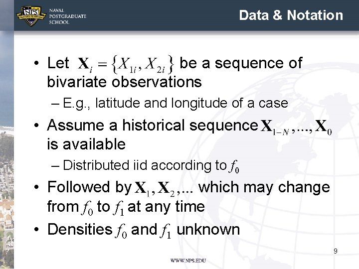
Data & Notation • Let be a sequence of bivariate observations – E. g. , latitude and longitude of a case • Assume a historical sequence is available – Distributed iid according to f 0 • Followed by which may change from f 0 to f 1 at any time • Densities f 0 and f 1 unknown 9

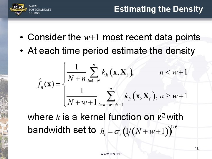
Estimating the Density • Consider the w+1 most recent data points • At each time period estimate the density where k is a kernel function on R 2 with bandwidth set to 10

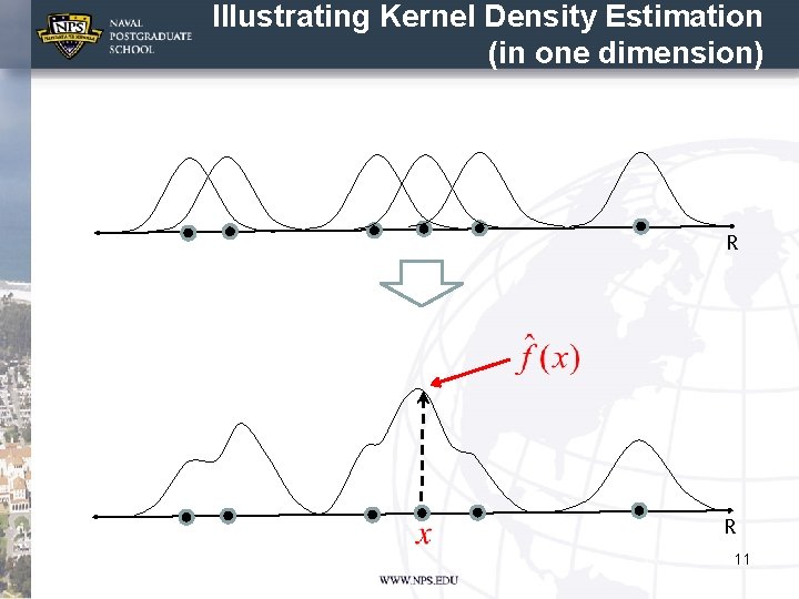
Illustrating Kernel Density Estimation (in one dimension) R R 11

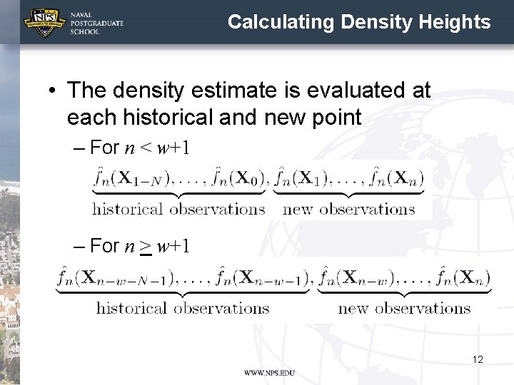
Calculating Density Heights • The density estimate is evaluated at each historical and new point – For n < w+1 – For n > w+1 12

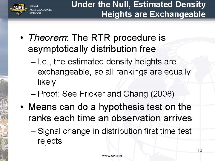
Under the Null, Estimated Density Heights are Exchangeable • Theorem: The RTR procedure is asymptotically distribution free – I. e. , the estimated density heights are exchangeable, so all rankings are equally likely – Proof: See Fricker and Chang (2008) • Means can do a hypothesis test on the ranks each time an observation arrives – Signal change in distribution first time test rejects 13

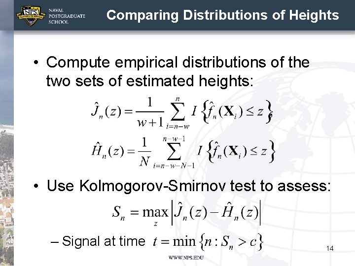
Comparing Distributions of Heights • Compute empirical distributions of the two sets of estimated heights: • Use Kolmogorov-Smirnov test to assess: – Signal at time 14

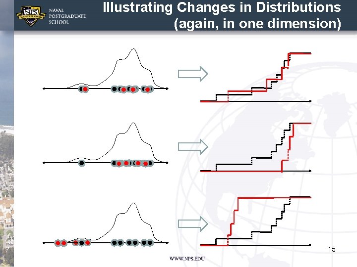
Illustrating Changes in Distributions (again, in one dimension) 15

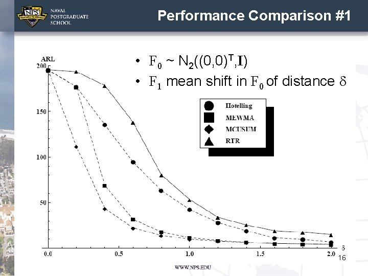
Performance Comparison #1 • F 0 ~ N 2((0, 0)T, I) • F 1 mean shift in F 0 of distance d 16

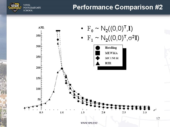
Performance Comparison #2 • F 0 ~ N 2((0, 0)T, I) • F 1 ~ N 2((0, 0)T, s 2 I) 17

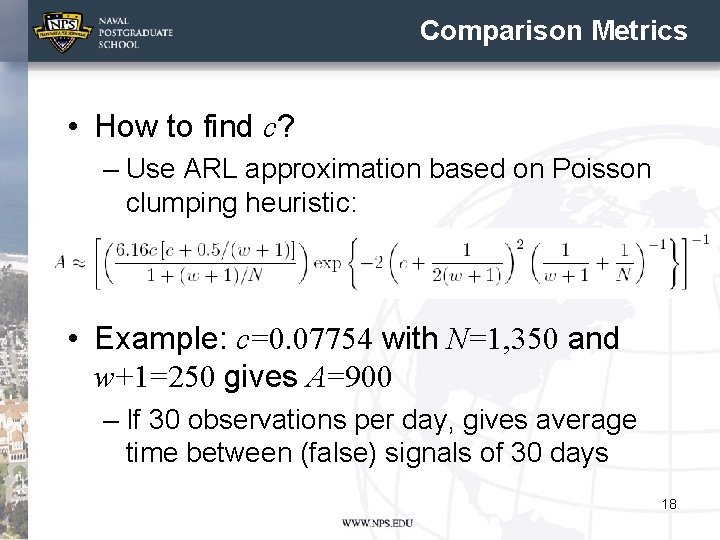
Comparison Metrics • How to find c? – Use ARL approximation based on Poisson clumping heuristic: • Example: c=0. 07754 with N=1, 350 and w+1=250 gives A=900 – If 30 observations per day, gives average time between (false) signals of 30 days 18

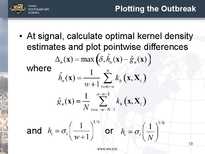
Plotting the Outbreak • At signal, calculate optimal kernel density estimates and plot pointwise differences where and or 19

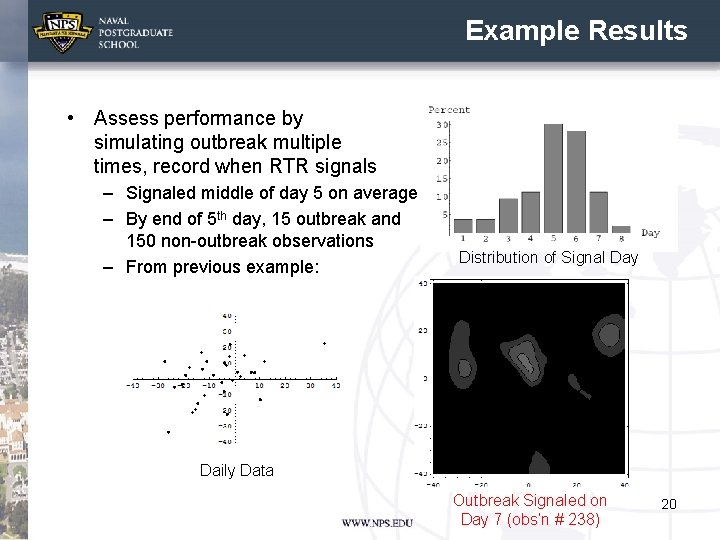
Example Results • Assess performance by simulating outbreak multiple times, record when RTR signals – Signaled middle of day 5 on average – By end of 5 th day, 15 outbreak and 150 non-outbreak observations – From previous example: Distribution of Signal Day Daily Data Outbreak Signaled on Day 7 (obs’n # 238) 20

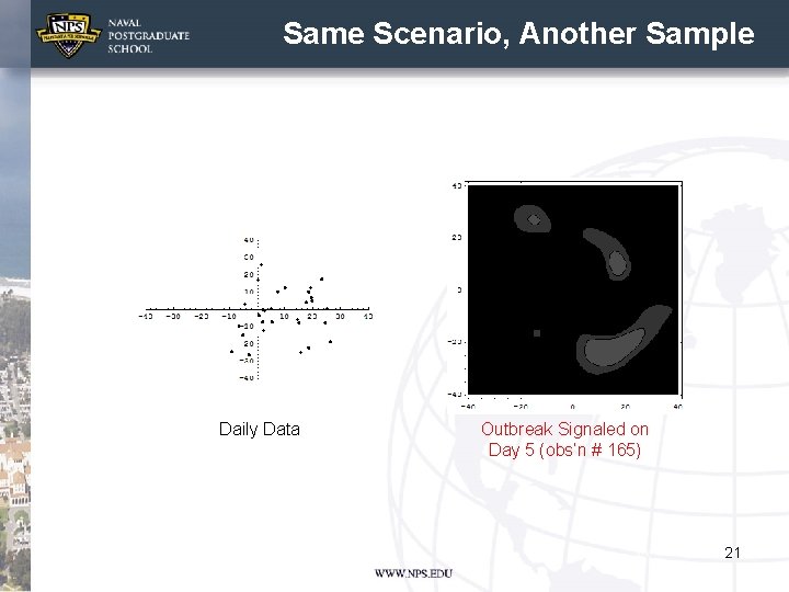
Same Scenario, Another Sample Daily Data Outbreak Signaled on Day 5 (obs’n # 165) 21

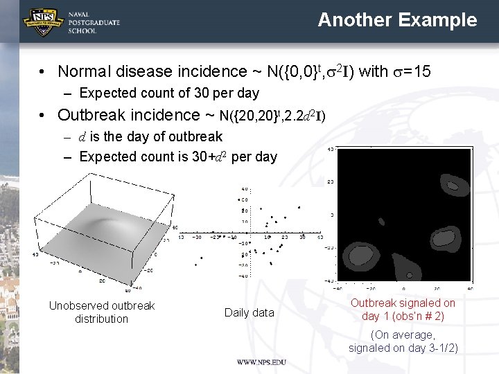
Another Example • Normal disease incidence ~ N({0, 0}t, s 2 I) with s=15 – Expected count of 30 per day • Outbreak incidence ~ N({20, 20}t, 2. 2 d 2 I) – d is the day of outbreak – Expected count is 30+d 2 per day Unobserved outbreak distribution Daily data Outbreak signaled on day 1 (obs’n # 2) (On average, signaled on day 3 -1/2)

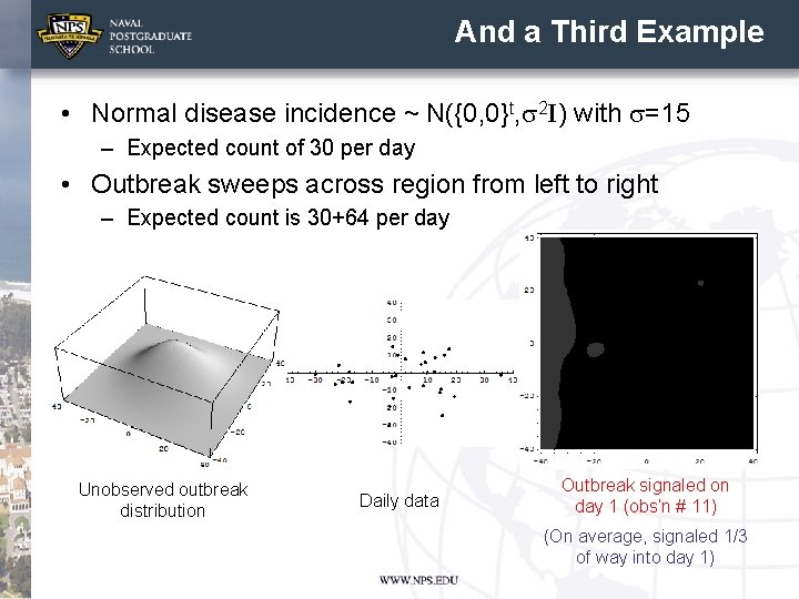
And a Third Example • Normal disease incidence ~ N({0, 0}t, s 2 I) with s=15 – Expected count of 30 per day • Outbreak sweeps across region from left to right – Expected count is 30+64 per day Unobserved outbreak distribution Daily data Outbreak signaled on day 1 (obs’n # 11) (On average, signaled 1/3 of way into day 1)

Advantages and Disadvantages • Advantages – Methodology supports both biosurveillance goals: early event detection and situational awareness – Incorporates observations sequentially (singly) • Most other methods use aggregated data – Can be used for more than two dimensions • Disadvantage? – Can’t distinguish increase distributed according to f 0 • Unlikely for bioterrorism attack? • Won’t detect an general increase in background disease incidence rate – E. g. , Perhaps caused by an increase in population – In this case, advantage not to detect 24

Selected References Detection Algorithm Development and Assessment: • Fricker, R. D. , Jr. , and J. T. Chang, The Repeated Two-Sample Rank Procedure: A Multivariate Nonparametric Individuals Control Chart (in draft). • Fricker, R. D. , Jr. , and J. T. Chang, A Spatio-temporal Method for Real-time Biosurveillance, Quality Engineering (to appear, November 2008). • Fricker, R. D. , Jr. , Knitt, M. C. , and C. X. Hu, Comparing Directionally Sensitive MCUSUM and MEWMA Procedures with Application to Biosurveillance, Quality Engineering (to appear, November 2008). • Joner, M. D. , Jr. , Woodall, W. H. , Reynolds, M. R. , Jr. , and R. D. Fricker, Jr. , A One-Sided MEWMA Chart for Health Surveillance, Quality and Reliability Engineering International, 24, pp. 503 -519, 2008. • Fricker, R. D. , Jr. , Hegler, B. L. , and D. A Dunfee, Assessing the Performance of the Early Aberration Reporting System (EARS) Syndromic Surveillance Algorithms, Statistics in Medicine, 27, pp. 3407 -3429, 2008. • Fricker, R. D. , Jr. , Directionally Sensitive Multivariate Statistical Process Control Methods with Application to Syndromic Surveillance, Advances in Disease Surveillance, 3: 1, 2007. Biosurveillance System Optimization: • Fricker, R. D. , Jr. , and D. Banschbach, Optimizing a System of Threshold Detection Sensors, in submission. Background Information: • Fricker, R. D. , Jr. , and H. Rolka, Protecting Against Biological Terrorism: Statistical Issues in Electronic Biosurveillance, Chance, 91, pp. 4 -13, 2006 • Fricker, R. D. , Jr. , Syndromic Surveillance, in Encyclopedia of Quantitative Risk Assessment, Melnick, E. , and Everitt, B (eds. ), John Wiley & Sons Ltd, pp. 1743 -1752, 2008. 25