Department of Informatics T E I of Athens

Department of Informatics, T. E. I. of Athens SELF-ORGANIZING MAPS: THEORY AND APPLICATIONS TO IMAGE COMPRESSION AND EFFICIENT CLASSIFICATION 2/22/2021 Nikolaos Vassilas 1

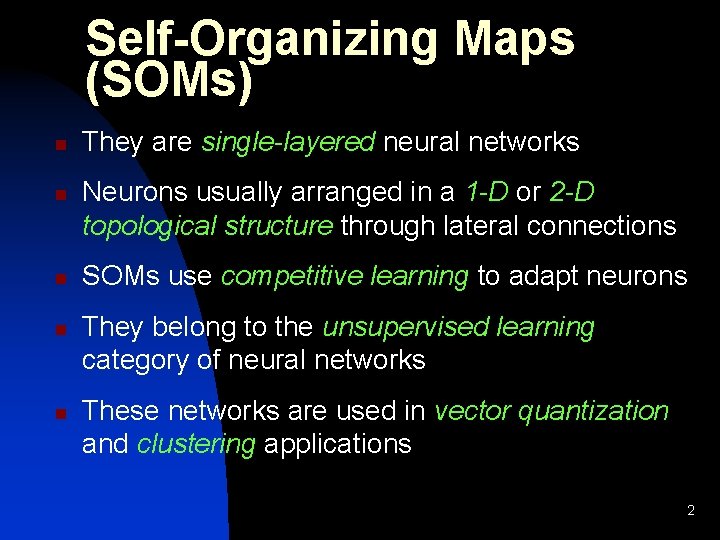
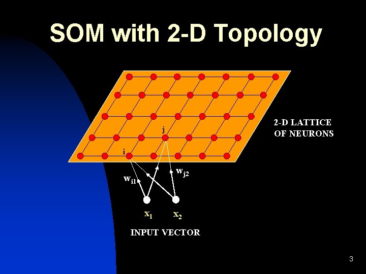
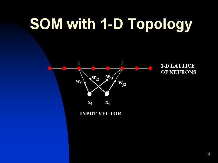
Self-Organizing Maps (SOMs) n n n They are single-layered neural networks Neurons usually arranged in a 1 -D or 2 -D topological structure through lateral connections SOMs use competitive learning to adapt neurons They belong to the unsupervised learning category of neural networks These networks are used in vector quantization and clustering applications 2

SOM with 2 -D Topology 2 -D LATTICE OF NEURONS j i wj 2 wi 1 x 2 INPUT VECTOR 3

SOM with 1 -D Topology j i wi 1 j wi 2 x 1 wj 1 1 -D LATTICE OF NEURONS wj 2 x 2 INPUT VECTOR 4

Winner Selection n Let x = (x 1, x 2, . . . , xn)T be the input vector in Rn n To each neuron i = (i 1, i 2) an associated weight vector wi = (wi 1, wi 2, . . . , win)T Rn n Neuron c = (c 1, c 2) whose weight vector wc is closest to the input (e. g. in Euclidean distance sense) is termed the winner of the competition: c = arg min {||x – wi||} i 5

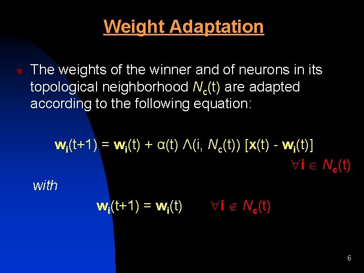
Weight Adaptation n The weights of the winner and of neurons in its topological neighborhood Nc(t) are adapted according to the following equation: wi(t+1) = wi(t) + α(t) Λ(i, Nc(t)) [x(t) - wi(t)] i Nc(t) with wi(t+1) = wi(t) i Nc(t) 6

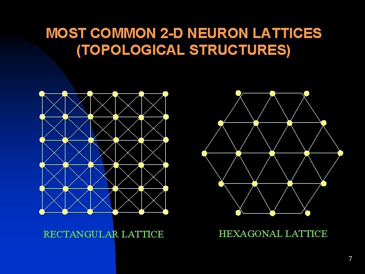
MOST COMMON 2 -D NEURON LATTICES (TOPOLOGICAL STRUCTURES) RECTANGULAR LATTICE HEXAGONAL LATTICE 7

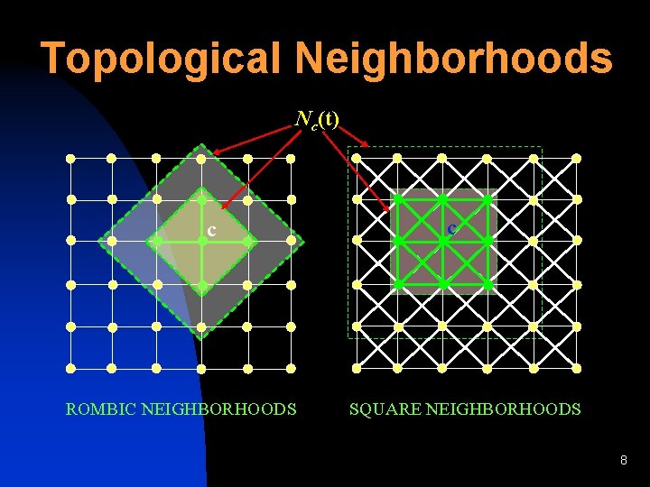
Topological Neighborhoods Nc(t) c ROMBIC NEIGHBORHOODS c SQUARE NEIGHBORHOODS 8

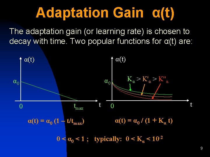
Adaptation Gain α(t) The adaptation gain (or learning rate) is chosen to decay with time. Two popular functions for α(t) are: α(t) Kα > K''α α 0 0 tmax α(t) = α 0 (1 – t/tmax) t t 0 α(t) = α 0 / (1 + Kα t) 0 < α 0 < 1 ; typically: 0 < Kα < 10 -2 9

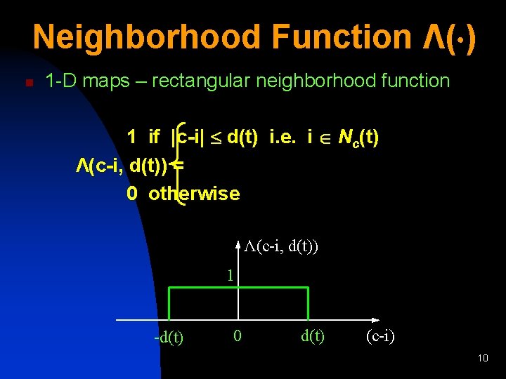
Neighborhood Function Λ( ) n 1 -D maps – rectangular neighborhood function 1 if |c-i| d(t) i. e. i Nc(t) Λ(c-i, d(t)) = 0 otherwise Λ(c-i, d(t)) 1 -d(t) 0 d(t) (c-i) 10

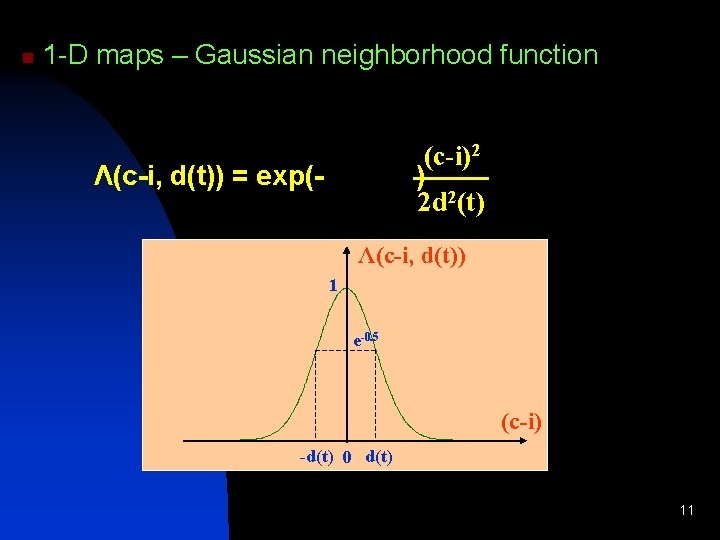
n 1 -D maps – Gaussian neighborhood function (c-i)2 ) 2 d 2(t) Λ(c-i, d(t)) = exp(- Λ(c-i, d(t)) 1 e-0. 5 (c-i) -d(t) 0 d(t) 11

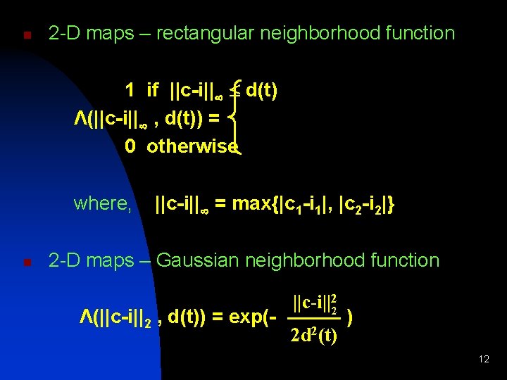
n 2 -D maps – rectangular neighborhood function 1 if ||c-i|| d(t) Λ(||c-i|| , d(t)) = 0 otherwise where, n ||c-i|| = max{|c 1 -i 1|, |c 2 -i 2|} 2 -D maps – Gaussian neighborhood function Λ(||c-i||2 , d(t)) = exp(- ||c-i||22 2 d 2(t) ) 12

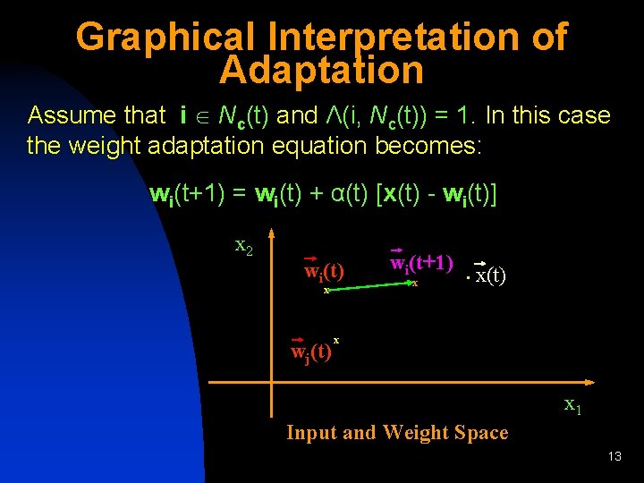
Graphical Interpretation of Adaptation Assume that i Nc(t) and Λ(i, Nc(t)) = 1. In this case the weight adaptation equation becomes: wi(t+1) = wi(t) + α(t) [x(t) - wi(t)] x 2 wi(t) x wj(t) wi(t+1) x • x(t) x x 1 Input and Weight Space 13

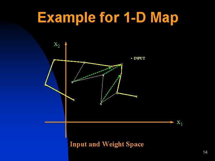
Example for 1 -D Map x 2 x • INPUT x x x 1 Input and Weight Space 14

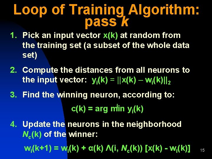
Loop of Training Algorithm: pass k 1. Pick an input vector x(k) at random from the training set (a subset of the whole data set) 2. Compute the distances from all neurons to the input vector: yi(k) = ||x(k) – wi(k)||2 3. Find the winning neuron, according to: i c(k) = arg min yi(k) 4. Update the neurons in the neighborhood Nc(k) of the winner: wi(k+1) = wi(k) + α(k) Λ(i, Nc(k)) [x(k) - wi(k)] 15

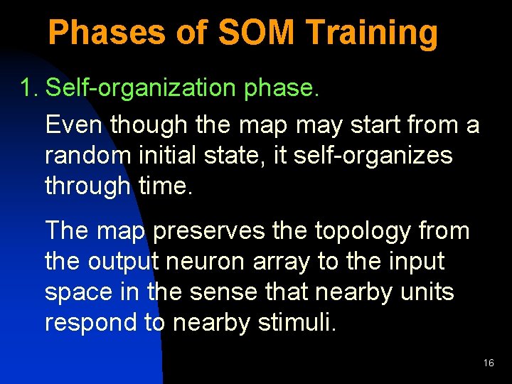
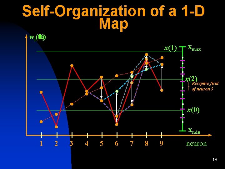
Phases of SOM Training 1. Self-organization phase. Even though the map may start from a random initial state, it self-organizes through time. The map preserves the topology from the output neuron array to the input space in the sense that nearby units respond to nearby stimuli. 16

2. Convergence phase. During this phase the weight vectors tend towards their asymptotic values and reproduce the input probability distribution as closely as possible. This phase has a much longer duration than self-organization. 17

Self-Organization of a 1 -D Map (1) (2) ( ) wi(0) x(1) xmax x(2) Receptive field of neuron 5 x(0) xmin 1 2 3 4 5 6 7 8 9 neuron 18

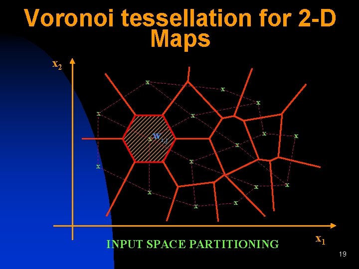
Voronoi tessellation for 2 -D Maps x 2 x x x x wi, j x x x x x INPUT SPACE PARTITIONING x 1 19

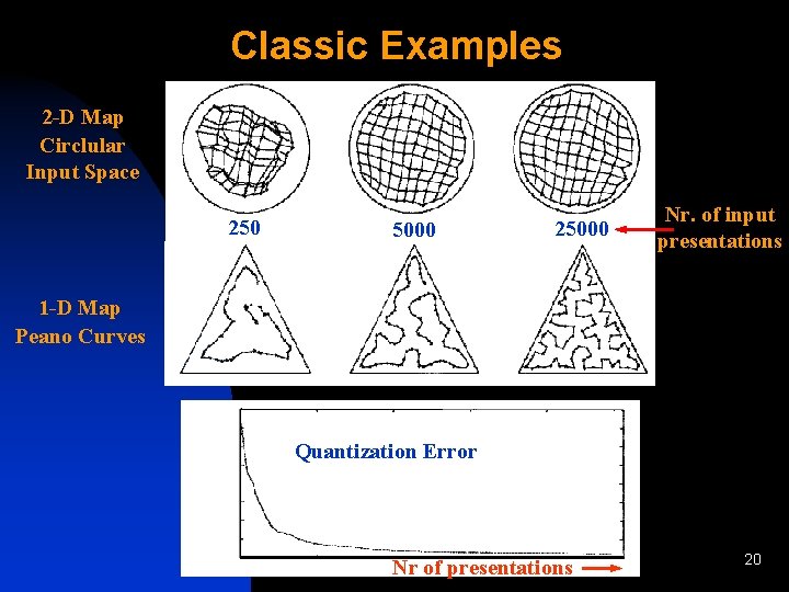
Classic Examples 2 -D Map Circlular Input Space 250 5000 25000 Nr. of input presentations 1 -D Map Peano Curves Quantization Error Nr of presentations 20

SOM Applications to Remotely-Sensed Data Compression and Classification 21

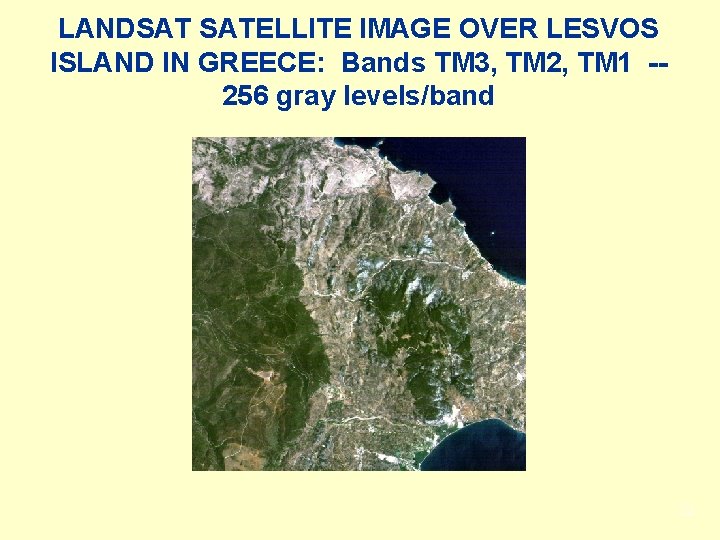
LANDSAT SATELLITE IMAGE OVER LESVOS ISLAND IN GREECE: Bands TM 3, TM 2, TM 1 -256 gray levels/band 22

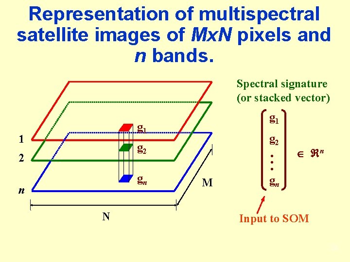
Representation of multispectral satellite images of Mx. N pixels and n bands. Spectral signature (or stacked vector) g 1 1 g 2 2 gn n N M n gn Input to SOM 23

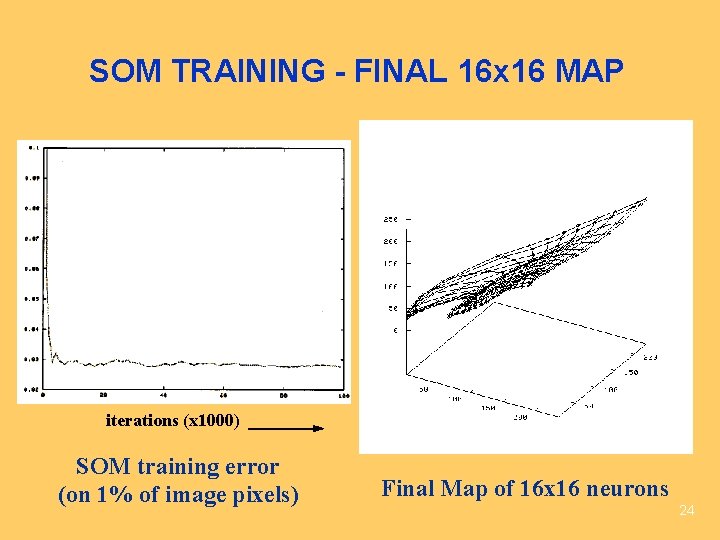
SOM TRAINING - FINAL 16 x 16 MAP iterations (x 1000) SOM training error (on 1% of image pixels) Final Map of 16 x 16 neurons 24

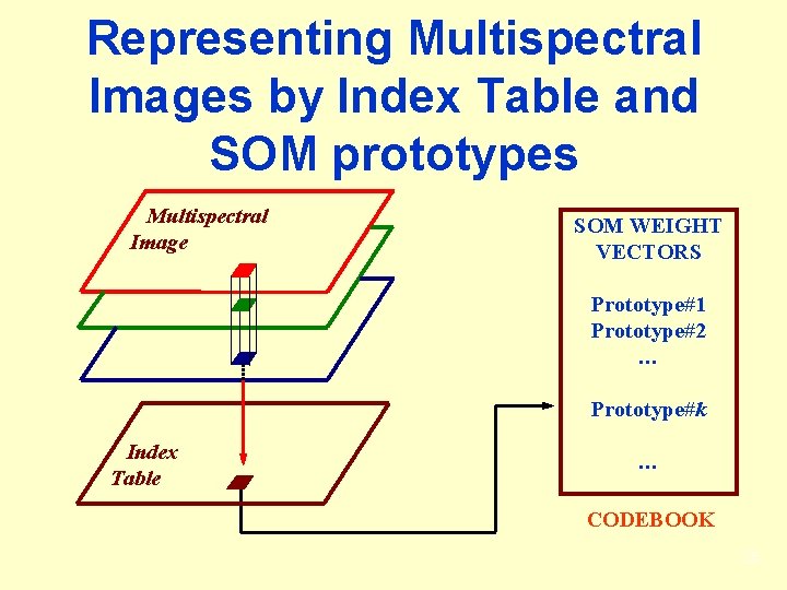
Representing Multispectral Images by Index Table and SOM prototypes Multispectral Image SOM WEIGHT VECTORS Prototype#1 Prototype#2 … Prototype#k Index Table … CODEBOOK 25

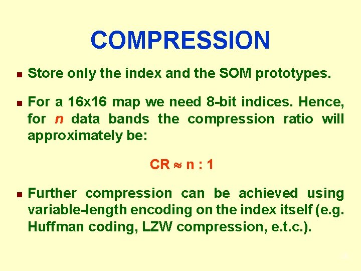
COMPRESSION n n Store only the index and the SOM prototypes. For a 16 x 16 map we need 8 -bit indices. Hence, for n data bands the compression ratio will approximately be: CR n : 1 n Further compression can be achieved using variable-length encoding on the index itself (e. g. Huffman coding, LZW compression, e. t. c. ). 26

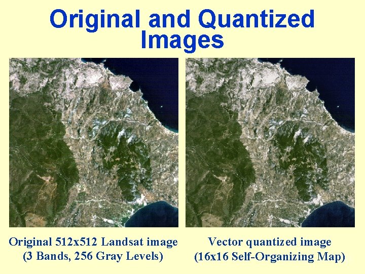
Original and Quantized Images Original 512 x 512 Landsat image (3 Bands, 256 Gray Levels) Vector quantized image (16 x 16 Self-Organizing Map)27

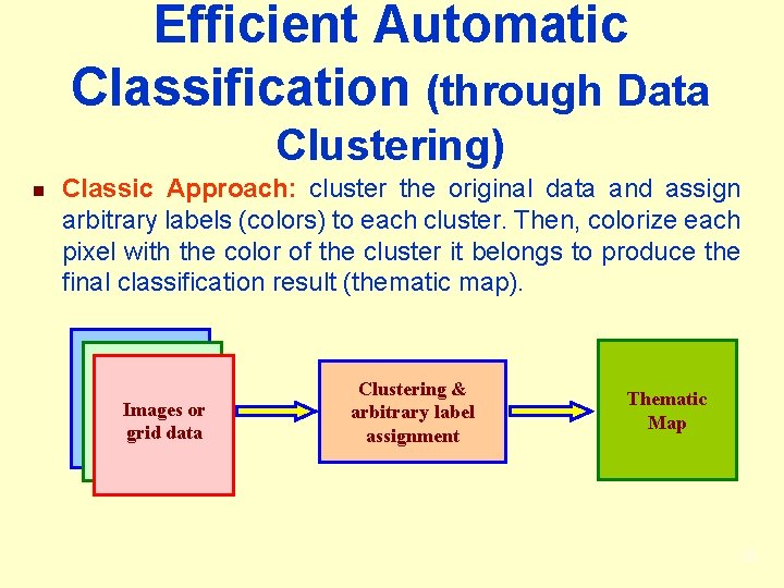
Efficient Automatic Classification (through Data Clustering) n Classic Approach: cluster the original data and assign arbitrary labels (colors) to each cluster. Then, colorize each pixel with the color of the cluster it belongs to produce the final classification result (thematic map). Images or grid data Clustering & arbitrary label assignment Thematic Map 28

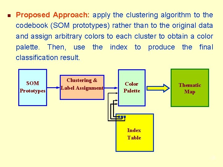
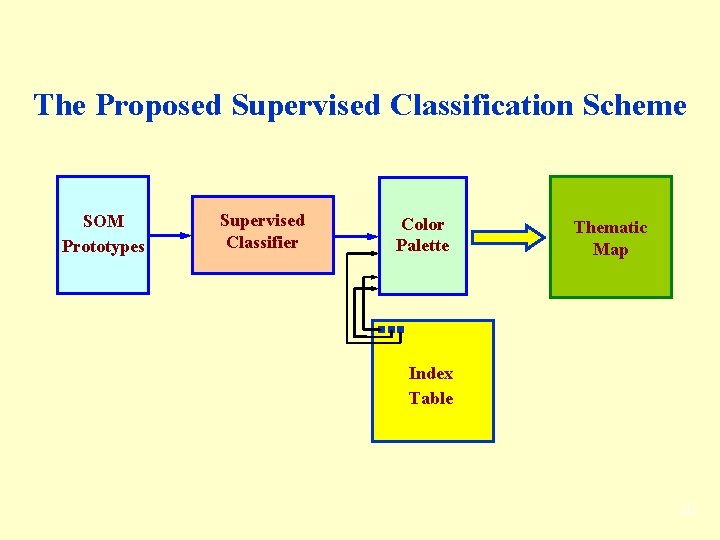
n Proposed Approach: apply the clustering algorithm to the codebook (SOM prototypes) rather than to the original data and assign arbitrary colors to each cluster to obtain a color palette. Then, use the index to produce the final classification result. SOM Prototypes Clustering & Label Assignment Color Palette Thematic Map Index Table 29

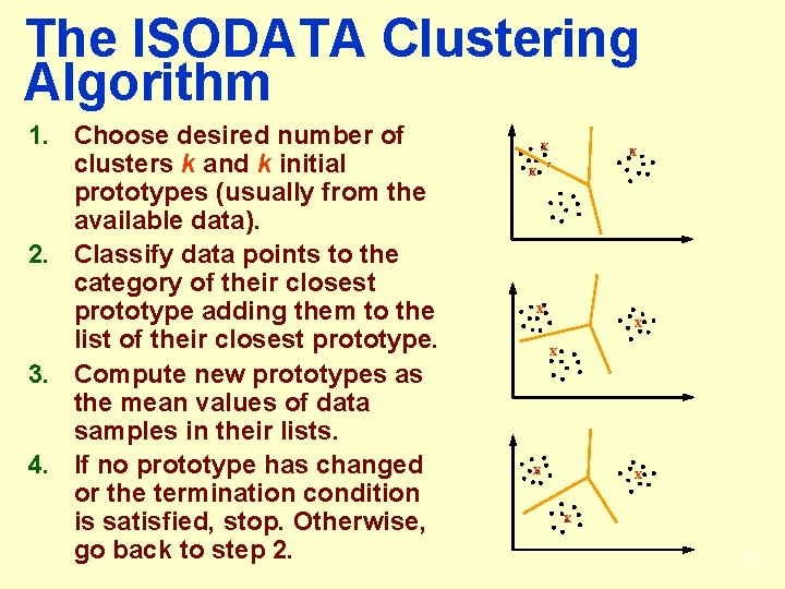
The ISODATA Clustering Algorithm 1. Choose desired number of clusters k and k initial prototypes (usually from the available data). 2. Classify data points to the category of their closest prototype adding them to the list of their closest prototype. 3. Compute new prototypes as the mean values of data samples in their lists. 4. If no prototype has changed or the termination condition is satisfied, stop. Otherwise, go back to step 2. x x x x x 30

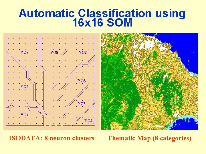
Automatic Classification using 16 x 16 SOM ISODATA: 8 neuron clusters Thematic Map (8 categories) 31

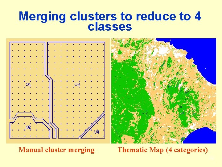
Merging clusters to reduce to 4 classes Manual cluster merging Thematic Map (4 categories) 32

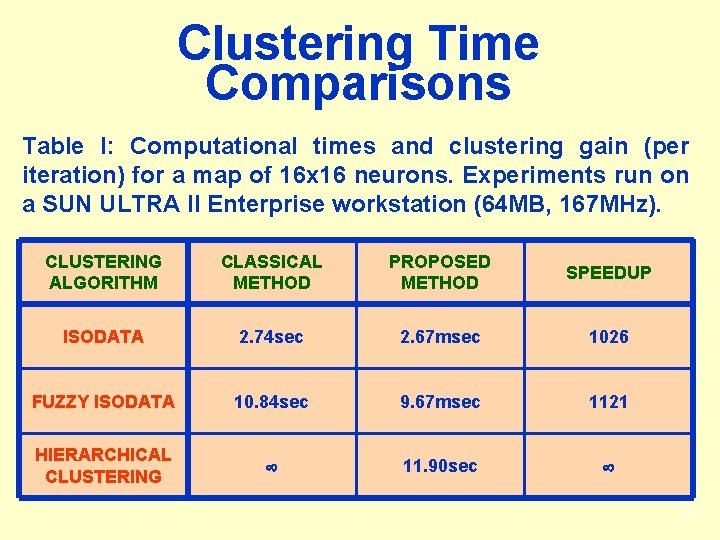
Clustering Time Comparisons Table I: Computational times and clustering gain (per iteration) for a map of 16 x 16 neurons. Experiments run on a SUN ULTRA II Enterprise workstation (64 MB, 167 MHz). CLUSTERING ALGORITHM CLASSICAL METHOD PROPOSED METHOD SPEEDUP ISODATA 2. 74 sec 2. 67 msec 1026 FUZZY ISODATA 10. 84 sec 9. 67 msec 1121 HIERARCHICAL CLUSTERING 11. 90 sec 33

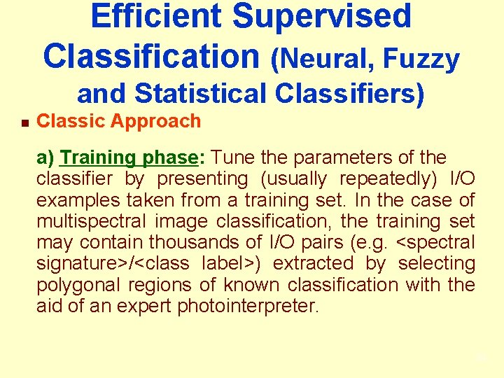
Efficient Supervised Classification (Neural, Fuzzy and Statistical Classifiers) n Classic Approach a) Training phase: Tune the parameters of the classifier by presenting (usually repeatedly) I/O examples taken from a training set. In the case of multispectral image classification, the training set may contain thousands of I/O pairs (e. g. <spectral signature>/<class label>) extracted by selecting polygonal regions of known classification with the aid of an expert photointerpreter. 34

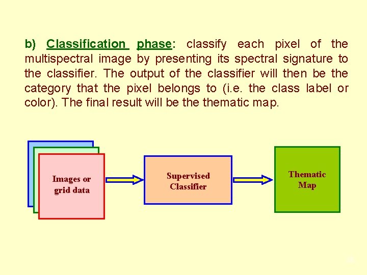
b) Classification phase: classify each pixel of the multispectral image by presenting its spectral signature to the classifier. The output of the classifier will then be the category that the pixel belongs to (i. e. the class label or color). The final result will be thematic map. Images or grid data Supervised Classifier Thematic Map 35

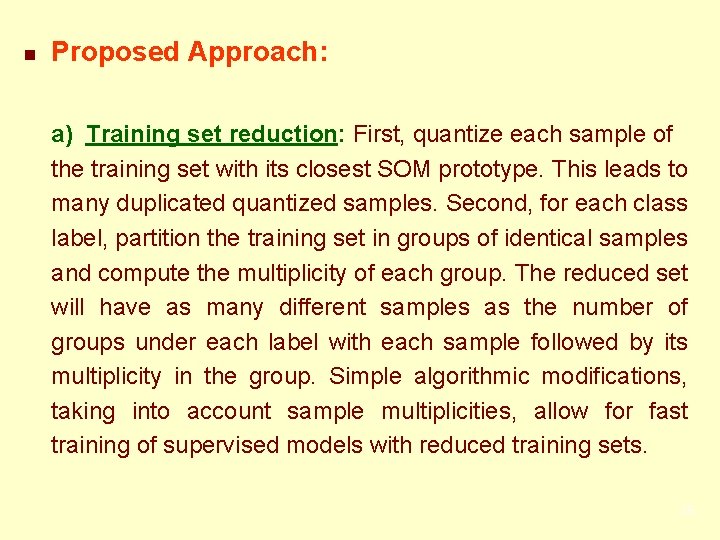
n Proposed Approach: a) Training set reduction: First, quantize each sample of the training set with its closest SOM prototype. This leads to many duplicated quantized samples. Second, for each class label, partition the training set in groups of identical samples and compute the multiplicity of each group. The reduced set will have as many different samples as the number of groups under each label with each sample followed by its multiplicity in the group. Simple algorithmic modifications, taking into account sample multiplicities, allow for fast training of supervised models with reduced training sets. 36

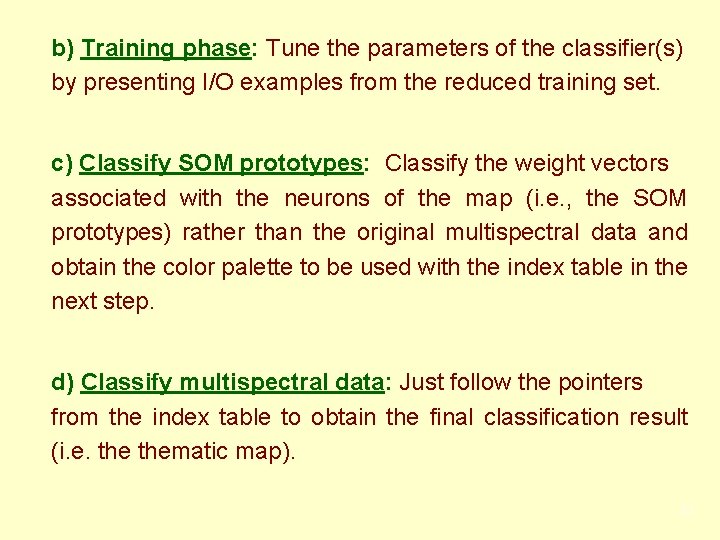
b) Training phase: Tune the parameters of the classifier(s) by presenting I/O examples from the reduced training set. c) Classify SOM prototypes: Classify the weight vectors associated with the neurons of the map (i. e. , the SOM prototypes) rather than the original multispectral data and obtain the color palette to be used with the index table in the next step. d) Classify multispectral data: Just follow the pointers from the index table to obtain the final classification result (i. e. thematic map). 37

The Proposed Supervised Classification Scheme SOM Prototypes Supervised Classifier Color Palette Thematic Map Index Table 38

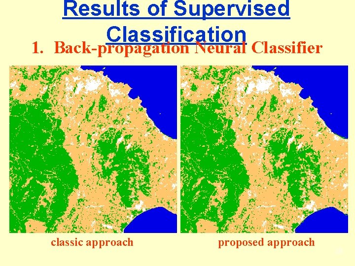
Results of Supervised Classification 1. Back-propagation Neural Classifier classic approach proposed approach 39

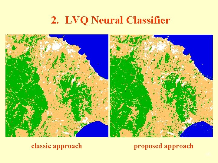
2. LVQ Neural Classifier classic approach proposed approach 40

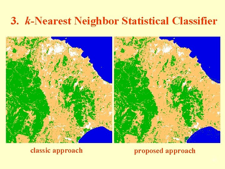
3. k-Nearest Neighbor Statistical Classifier classic approach proposed approach 41

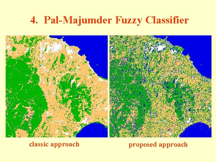
4. Pal-Majumder Fuzzy Classifier classic approach proposed approach 42

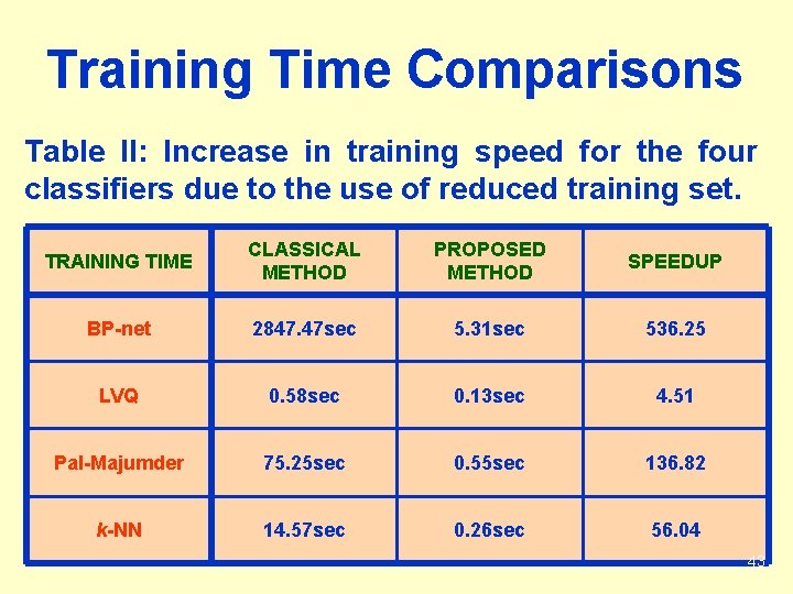
Training Time Comparisons Table II: Increase in training speed for the four classifiers due to the use of reduced training set. TRAINING TIME CLASSICAL METHOD PROPOSED METHOD SPEEDUP BP-net 2847. 47 sec 5. 31 sec 536. 25 LVQ 0. 58 sec 0. 13 sec 4. 51 Pal-Majumder 75. 25 sec 0. 55 sec 136. 82 k-NN 14. 57 sec 0. 26 sec 56. 04 43

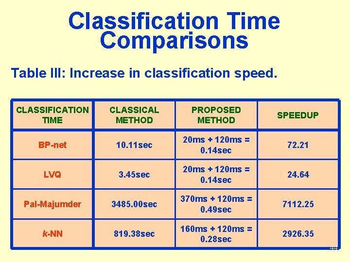
Classification Time Comparisons Table III: Increase in classification speed. CLASSIFICATION TIME CLASSICAL METHOD PROPOSED METHOD SPEEDUP BP-net 10. 11 sec 20 ms + 120 ms = 0. 14 sec 72. 21 LVQ 3. 45 sec 20 ms + 120 ms = 0. 14 sec 24. 64 Pal-Majumder 3485. 00 sec 370 ms + 120 ms = 0. 49 sec 7112. 25 k-NN 819. 38 sec 160 ms + 120 ms = 0. 28 sec 2926. 35 44

EPILOGUE Using classical clustering and/or classification algorithms on vast amount of data such as multisource remotely sensed data may not be a wise thing to do. For such data, the use of speedy techniques that involve vector quantization of the input space is strongly recommended. 45