DCSP10 Applications Jianfeng Feng Department of Computer Science

Applications • Power spectrum estimate • Image • Sampling theorem

Applications • Power spectrum estimate • Compression • Image • Sampling theorem

Understanding the plot • Sampling rate is Fs, the largest (fastest) frequency from the

Spectrogram • In real life example, all signals change with time (music for example)

A Matlab Example Three signals • • • • • • • • •

• • A Matlab Example Original signal + disturbance + noise • •

A Matlab Example • Will come back to it in the next few weeks

Issues on noise • Two sets of random noise (100 points each, upper panel)

Issues on noise • Taking expectation abs (DFT ( {x[n], n=0, …, N-1} )

Issues on noise • Remember that the ACF of white noise is • Powers

Issues on noise light goes a through a prism White light. White passes prism

Image Processing • two-dimensional signal x[n 1, n 2], n 1, n 2∈Z •

Image Processing • Gray scale images: scalar pixel values • color images: multidimensional pixel

Example I clear all close all figure(1) I = imread('peppers. png'); imshow(I); K=rgb 2

Example I FF=(100*log(1+abs(fftshift(F)))); for i=1: 384 for j=1: 512 ss=sqrt((i-192)*(i-192)+(j-256)*(j-256)); if(ss>100) FF(i, j)=0; end

Example I ? FF=(100*log(1+abs(fftshift(F)))); for i=1: 384 for j=1: 512 ss=sqrt((i-192)*(i-192)+(j-256)*(j-256)); if(ss>100) FF(i, j)=0;

Sampling and reconstruction The question we consider here is under what conditions we can

Sampling and reconstruction Theorem (Nyquist-Shannon sampling thm) Exact reconstruction of a continuous-time signal from

Summary of FT • At the end of the day, FT for signal x

Filter • A filter is a device or process that removes from a signal

A Filter will look like this Received signal x [n] (lifted it up for

A Filter will look like this y ([i] = ( x[i] +…+x [i-N]) /

A Filter will look like this You might be able to guess what is

Filter In general, we can include both the input x [n-k] and the previous

Example • In this case, when bi=0, it is an MA y(n) = [

Slides: 44

Download presentation

DCSP-10: Applications Jianfeng Feng Department of Computer Science Warwick Univ. , UK Jianfeng@warwick. ac. uk http: //www. dcs. warwick. ac. uk/~feng/dcsp. html

Applications • Power spectrum estimate • Image • Sampling theorem

Spectrogram: real life example

Applications • Power spectrum estimate • Compression • Image • Sampling theorem

Understanding the plot • Sampling rate is Fs, the largest (fastest) frequency from the data is then Fs/2 • Remembering that our frequency domain is in [0 2 p] which matches to [0 Fs] • Divide [0 Fs] into N intervals and plot abs X[k] against k. Fs/N which gives power against frequency • Since it is symmetric, we sometime only plot out [0, Fs//2] Here Fs =1 0 Hz

Spectrogram • In real life example, all signals change with time (music for example) • Using sliding window to sample signals and calculate PSD -- STFT

A Matlab Example Three signals • • • • • • • • • • • • • close all clear all load handel; figure(1) plot(y); xlabel('time') T=size(y); for i=1: T(1, 1) fre_x(i)=i*Fs/T(1, 1); end figure(2) plot(fre_x, abs(fft(y))) xlabel('Hz') figure(3) spectrogram(y, 128, 120, [], Fs); • ; T 1=floor(T(1, 1)/2); omega 1=1000; for i=1: T(1, 1)-T 1; z(i, 1)=y(i, 1)+. 3*cos(2*pi*omega 1*i/Fs); end omega 2=2000; for i=T-T 1+1: T(1, 1); z(i, 1)=y(i, 1)+. 3*cos(2*pi*omega 2*i/Fs); end figure(5) plot(z); xlabel('time') figure(6) plot(fre_x, abs(fft(z))) xlabel('Hz') figure(7) spectrogram(z, 128, 120, [], Fs); for i=1: T(1, 1); zn(i, 1)=y(i, 1)+. 3*randn(1, 1); end figure(8) plot(zn); xlabel('time') figure(9) plot(fre_x, abs(fft(zn))) xlabel('Hz') figure(10) spectrogram(zn, 128, 120, [], Fs);

• • A Matlab Example Original signal + disturbance + noise • • • • • • • • • • • • close all clear all load handel; figure(1) plot(y); xlabel('time') T=size(y); for i=1: T(1, 1) fre_x(i)=i*Fs/T(1, 1); end figure(2) plot(fre_x, abs(fft(y))) xlabel('Hz') figure(3) spectrogram(y, 128, 120, [], Fs); • ; T 1=floor(T(1, 1)/2); omega 1=1000; for i=1: T(1, 1)-T 1; z(i, 1)=y(i, 1)+. 3*cos(2*pi*omega 1*i/Fs); end omega 2=2000; for i=T-T 1+1: T(1, 1); z(i, 1)=y(i, 1)+. 3*cos(2*pi*omega 2*i/Fs); end figure(5) plot(z); xlabel('time') figure(6) plot(fre_x, abs(fft(z))) xlabel('Hz') figure(7) spectrogram(z, 128, 120, [], Fs); for i=1: T(1, 1); zn(i, 1)=y(i, 1)+. 3*randn(1, 1); end figure(8) plot(zn); xlabel('time') figure(9) plot(fre_x, abs(fft(zn))) xlabel('Hz') figure(10) spectrogram(zn, 128, 120, [], Fs);

A Matlab Example • • • • • • • • • • • • • close all clear all load handel; figure(1) plot(y); xlabel('time') T=size(y); for i=1: T(1, 1) fre_x(i)=i*Fs/T(1, 1); end figure(2) plot(fre_x, abs(fft(y))) xlabel('Hz') figure(3) spectrogram(y, 128, 120, [], Fs); • ; T 1=floor(T(1, 1)/2); omega 1=1000; for i=1: T(1, 1)-T 1; z(i, 1)=y(i, 1)+. 3*cos(2*pi*omega 1*i/Fs); end omega 2=2000; for i=T-T 1+1: T(1, 1); z(i, 1)=y(i, 1)+. 3*cos(2*pi*omega 2*i/Fs); end figure(5) plot(z); xlabel('time') figure(6) plot(fre_x, abs(fft(z))) xlabel('Hz') figure(7) spectrogram(z, 128, 120, [], Fs); for i=1: T(1, 1); zn(i, 1)=y(i, 1)+. 3*randn(1, 1); end figure(8) plot(zn); xlabel('time') figure(9) plot(fre_x, abs(fft(zn))) xlabel('Hz') figure(10) spectrogram(zn, 128, 120, [], Fs); Abs(fft) vs Frequency

A Matlab Example • Will come back to it in the next few weeks after we learn how to design filters

Issues on noise • Two sets of random noise (100 points each, upper panel) • Power Spectrum (bottom panel) • Make sense?

Issues on noise • Taking expectation abs (DFT ( {x[n], n=0, …, N-1} ) ) E | (DFT ( {x[n], n=0, …, N-1} ) )| 2 = DFT ( {g [n] } ) where g [n] is the auto-correlation function (ACF) • Remember that the ACF of white noise is

Issues on noise • Remember that the ACF of white noise is • Powers are equally distributed at each frequency • Hence the name of ‘white noise’ • Colour noise: not equally distributed (ACF is not delta)

Issues on noise light goes a through a prism White light. White passes prism Remember that the ACF of white noise is • Powers are equally distributed at each frequency • Hence the name of ‘white noise’ • Colour noise: not equally distributed (ACF is not delta)

Image Processing • two-dimensional signal x[n 1, n 2], n 1, n 2∈Z • indices locate a point on a grid → pixel • grid is usually regularly spaced • values x[n 1, n 2] refer to the pixel’s appearance

Image Processing • Gray scale images: scalar pixel values • color images: multidimensional pixel values in a color space (RGB for example) • we can consider the single components separately:

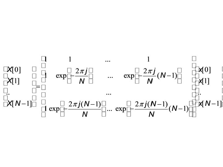
DFT for image • DFT for x • IDFT for X

Example I clear all close all figure(1) I = imread('peppers. png'); imshow(I); K=rgb 2 gray(I); figure(2) F = fft 2(K); figure; imagesc(100*log(1+abs(fftshift(F)))); colormap(gray); title('magnitude spectrum'); figure; imagesc(angle(F)); colormap(gray) Original picture Gray scale picture

Example I

Example I FF=(100*log(1+abs(fftshift(F)))); for i=1: 384 for j=1: 512 ss=sqrt((i-192)*(i-192)+(j-256)*(j-256)); if(ss>100) FF(i, j)=0; end end figure; imagesc(FF); colormap(gray); title('magnitude spectrum'); figure; imagesc(angle(FF)); colormap(gray) All low frequency information is here

Example I ? FF=(100*log(1+abs(fftshift(F)))); for i=1: 384 for j=1: 512 ss=sqrt((i-192)*(i-192)+(j-256)*(j-256)); if(ss>100) FF(i, j)=0; end end figure; imagesc(FF); colormap(gray); title('magnitude spectrum'); figure; imagesc(angle(FF)); colormap(gray) All high frequency information is here

Example II Image processing

Example III: mind reading IDFT 2

Sampling and reconstruction The question we consider here is under what conditions we can completely reconstruct the original signal x(t) from its discretely sampled signal x[n].

Sampling and reconstruction Theorem (Nyquist-Shannon sampling thm) Exact reconstruction of a continuous-time signal from its samples is possible if the signal is bandlimited and the sampling frequency is greater than twice the signal bandwidth Proof. The proof is again an application of FT, but we will not go through it here Please read around. It is based upon the sinc function.

Summary of FT • At the end of the day, FT for signal x is only fft(x) it is deadly easy • Hopefully and I am sure it will be useful for your future career

Summary of FT • At the end of the day, FT for signal x is only fft(x) it is deadly easy • Hopefully it will be useful for your future career • I am proud of this

Filter • A filter is a device or process that removes from a signal some unwanted component or feature. • Filtering is a class of signal processing, the defining feature of filters being the complete or partial suppression of some aspect of the signal. • Most often, this means removing some frequencies and not others in order to suppress interfering signals and reduce background noise.

Filter

A Filter will look like this Received signal x [n] (lifted it up for 5 units for visualization)

A Filter will look like this y ([i] = ( x[i] +…+x [i-N]) / (N+1) N=9 here

A Filter will look like this y ([i] = ( x[i] +…+x [i-N]) / ( N+1) N=9 here

A Filter will look like this y ([i] = ( x[i] +…+x [i-N]) / (N+1) N=9 here This filter is called moving average MA(10)

A Filter will look like this You might be able to guess what is the original signal

A Filter will look like this y ([i] = ( x[i] +…+x [i-N]) / (N+1) + (y[i-1]+…y[i-N])/N This filter is called auto-regressive moving average ARMA(p, q)

Filter In general, we can include both the input x [n-k] and the previous outputs y [n-k] to generate y(n) = a 0 x(n)+a 1 x(n-1)+…+a. Nx(n-N) +b 1 y(n-1)+…+b. Ny(n-N) N th order filter

Example • In this case, when bi=0, it is an MA y(n) = [ x(n)+ … x(n-N) ] / N • In general it is called ARMA filter. AR for auto-regressive