LogLinear Models Dependent Samples Feng Ye Xiao Guo

Log-Linear Models & Dependent Samples Feng Ye, Xiao Guo, Jing Wang

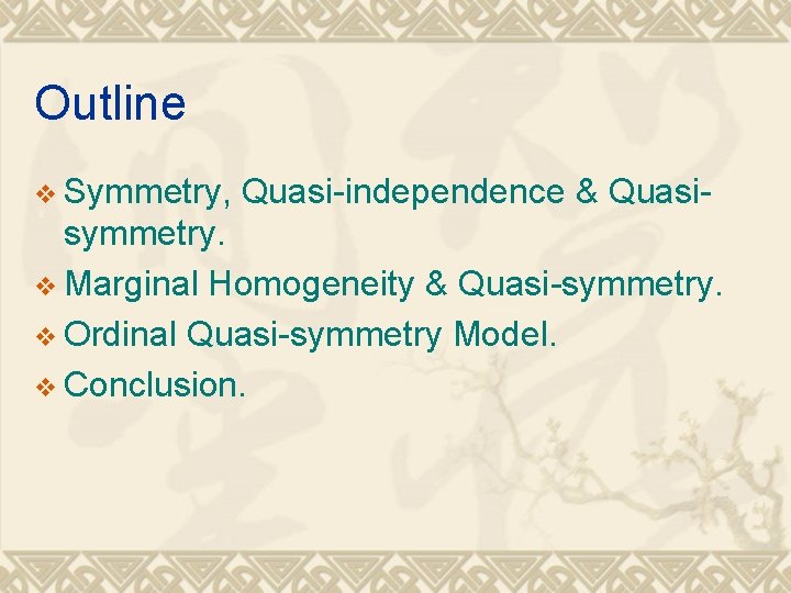
Outline v Symmetry, Quasi-independence & Quasi- symmetry. v Marginal Homogeneity & Quasi-symmetry. v Ordinal Quasi-symmetry Model. v Conclusion.

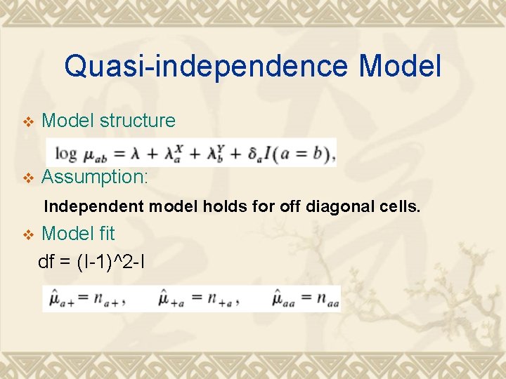
Quasi-independence Model v Model structure Assumption: Independent model holds for off diagonal cells. v Model fit df = (I-1)^2 -I v

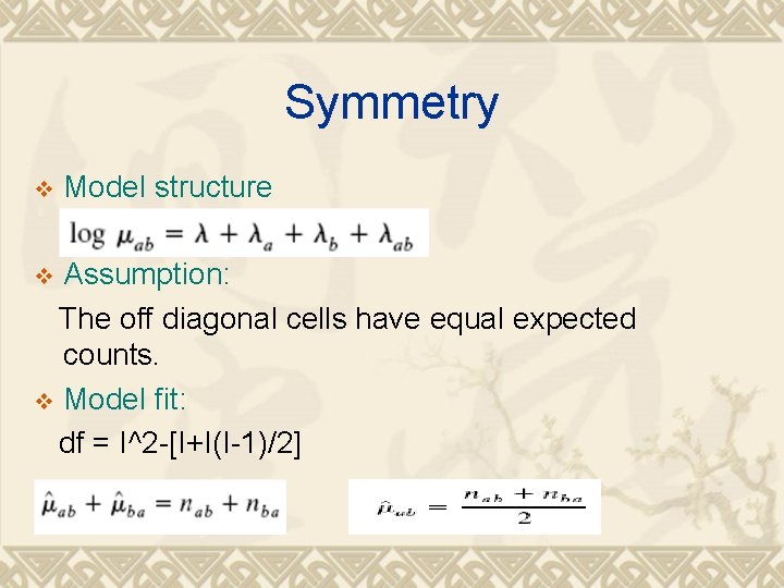
Symmetry v Model structure Assumption: The off diagonal cells have equal expected counts. v Model fit: df = I^2 -[I+I(I-1)/2] v

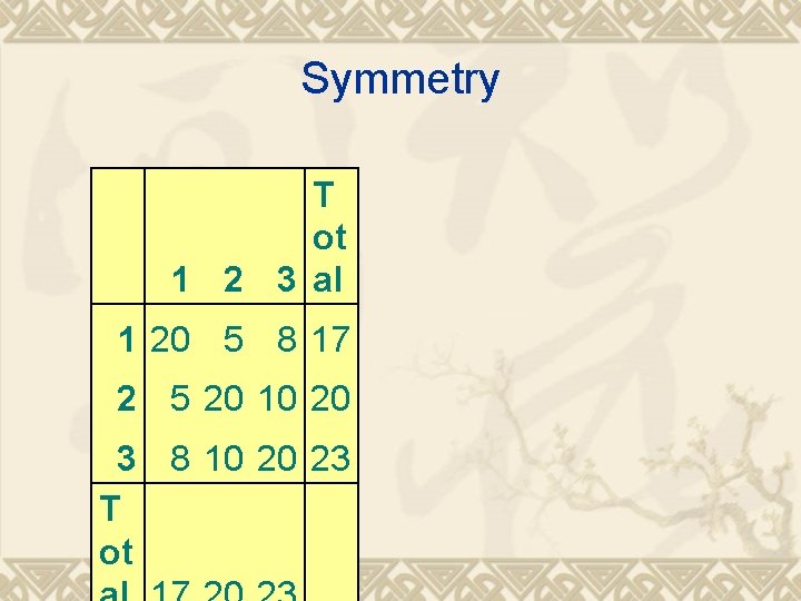
Symmetry T ot 1 2 3 al 1 20 5 8 17 2 5 20 10 20 3 8 10 20 23 T ot

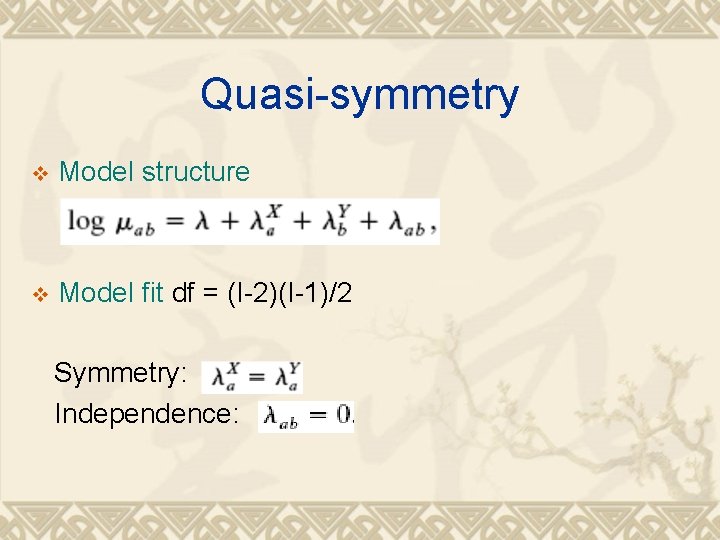
Quasi-symmetry v Model structure Model fit df = (I-2)(I-1)/2 Symmetry: Independence: v

Application v Each week Variety magazine summarizes reviews of new movies by critics in several cities. Each review is categorized as pro, con, or mixed, according to whether the overall evaluation is positive, negative, or a mixture of the two. April 1995 through September 1996 for Chicago film critics Gene Siskel and Roger Ebert.

Application v Reviews of new movies by critics. Eb ert Mi Sis Co xe Pr kel n d o Co n 24 8 13 Mi xe d 8 13 11

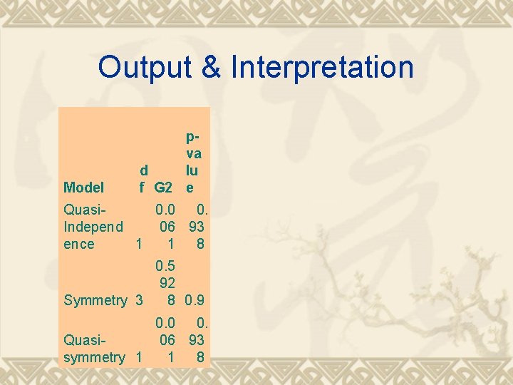
Output & Interpretation Model pva d lu f G 2 e Quasi 0. 0 0. Independ 06 93 ence 1 1 8 0. 5 92 Symmetry 3 8 0. 9 0. 0 0. Quasi 06 93 symmetry 1 1 8

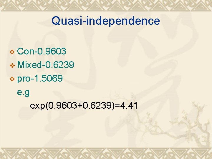
Quasi-independence v Con-0. 9603 v Mixed-0. 6239 v pro-1. 5069 e. g exp(0. 9603+0. 6239)=4. 41

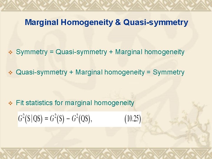
Marginal Homogeneity & Quasi-symmetry v Symmetry = Quasi-symmetry + Marginal homogeneity v Quasi-symmetry + Marginal homogeneity = Symmetry v Fit statistics for marginal homogeneity

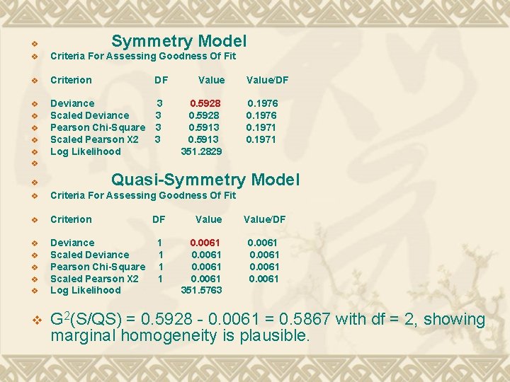
Symmetry Model v Criteria For Assessing Goodness Of Fit v Criterion DF v Deviance Scaled Deviance Pearson Chi-Square Scaled Pearson X 2 Log Likelihood 3 3 v v v Value 0. 5928 0. 5913 351. 2829 Value/DF 0. 1976 0. 1971 v Quasi-Symmetry Model v v Criteria For Assessing Goodness Of Fit v Criterion v Deviance Scaled Deviance Pearson Chi-Square Scaled Pearson X 2 Log Likelihood v v v DF Value 1 1 0. 0061 351. 5763 Value/DF 0. 0061 G 2(S/QS) = 0. 5928 - 0. 0061 = 0. 5867 with df = 2, showing marginal homogeneity is plausible.

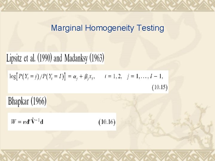
Marginal Homogeneity Testing

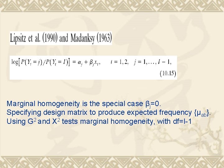
Marginal homogeneity is the special case βj=0. Specifying design matrix to produce expected frequency {µab}. Using G 2 and X 2 tests marginal homogeneity, with df=I-1

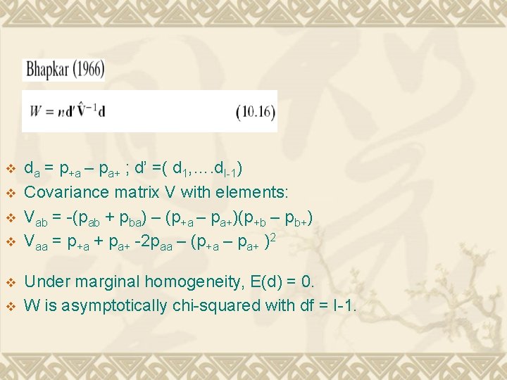
v v v da = p+a – pa+ ; d’ =( d 1, …. d. I-1) Covariance matrix V with elements: Vab = -(pab + pba) – (p+a – pa+)(p+b – pb+) Vaa = p+a + pa+ -2 paa – (p+a – pa+ )2 Under marginal homogeneity, E(d) = 0. W is asymptotically chi-squared with df = I-1.

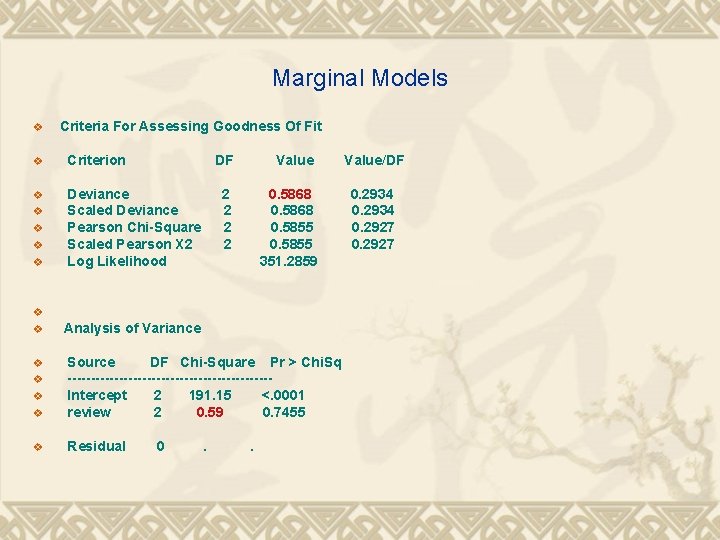
Marginal Models v Criteria For Assessing Goodness Of Fit v Criterion v Deviance Scaled Deviance Pearson Chi-Square Scaled Pearson X 2 Log Likelihood v v DF Value 2 2 0. 5868 0. 5855 351. 2859 v v Analysis of Variance v Source DF Chi-Square Pr > Chi. Sq ----------------------Intercept 2 191. 15 <. 0001 review 2 0. 59 0. 7455 v Residual v v v 0 . . Value/DF 0. 2934 0. 2927

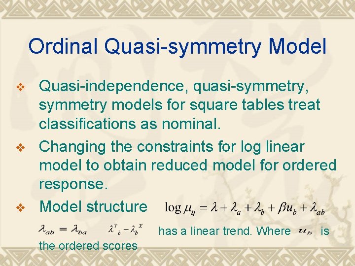
Ordinal Quasi-symmetry Model v v v Quasi-independence, quasi-symmetry, symmetry models for square tables treat classifications as nominal. Changing the constraints for log linear model to obtain reduced model for ordered response. Model structure has a linear trend. Where is the ordered scores

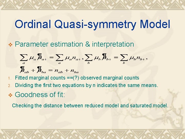
Ordinal Quasi-symmetry Model v Parameter estimation & interpretation 2. Fitted marginal counts ==(? ) observed marginal counts Dividing the first two equations by n indicates the same means. v Goodness of fit: 1. Checking the distance between reduced model and saturated model.

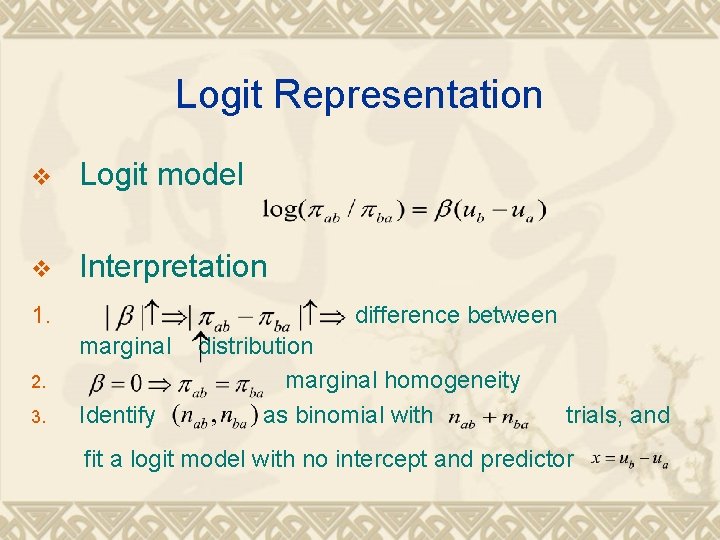
Logit Representation v Logit model v Interpretation difference between 1. 2. 3. marginal distribution marginal homogeneity Identify as binomial with trials, and fit a logit model with no intercept and predictor

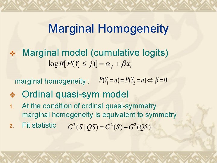
Marginal Homogeneity v Marginal model (cumulative logits) marginal homogeneity : v Ordinal quasi-sym model 1. 2. At the condition of ordinal quasi-symmetry marginal homogeneity is equivalent to symmetry Fit statistic

Application Data 1 v Reviews of new movies by critics. Eb ert Mi Sis Co xe Pr kel n d o Co n 24 8 13 Mi xe d 8 13 11

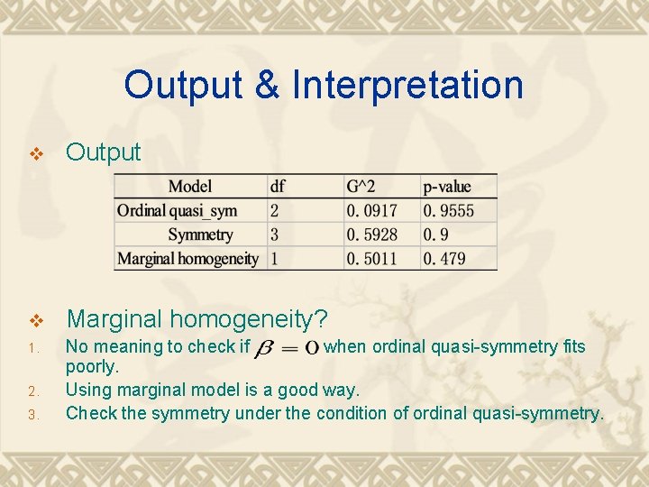
Output & Interpretation v Output v Marginal homogeneity? 1. No meaning to check if when ordinal quasi-symmetry fits poorly. Using marginal model is a good way. Check the symmetry under the condition of ordinal quasi-symmetry. 2. 3.

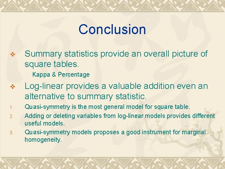
Conclusion v Summary statistics provide an overall picture of square tables. Kappa & Percentage v Log-linear provides a valuable addition even an alternative to summary statistic. 1. Quasi-symmetry is the most general model for square table. Adding or deleting variables from log-linear models provides different useful models. Quasi-symmetry models proposes a good instrument for marginal homogeneity. 2. 3.