DCSP17 Revision Jianfeng Feng Department of Computer Science

DCSP-17: Revision Jianfeng Feng Department of Computer Science Warwick Univ. , UK Jianfeng@warwick. ac. uk http: //www. dcs. warwick. ac. uk/~feng/dcsp. html

Today • • • I will go through the materials we learnt this term In particular, possible questions in exam Hope to see you all here • • Will have a revision class next term This week, on Monday and Thursday, we have assignment helps (will let you know the time late on) Assignment deadline is this Thursday at noon

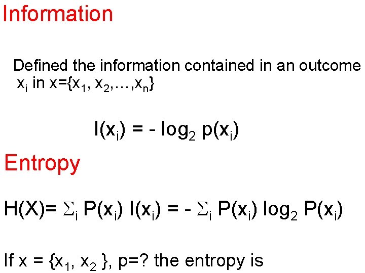
Information Defined the information contained in an outcome xi in x={x 1, x 2, …, xn} I(xi) = - log 2 p(xi) Entropy H(X)= Si P(xi) I(xi) = - Si P(xi) log 2 P(xi) If x = {x 1, x 2 }, p=? the entropy is

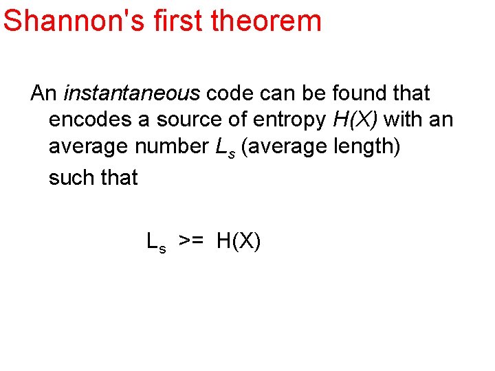
Shannon's first theorem An instantaneous code can be found that encodes a source of entropy H(X) with an average number Ls (average length) such that Ls >= H(X)

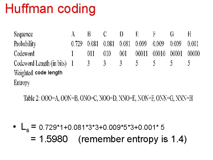
Huffman coding code length • Ls = 0. 729*1+0. 081*3*3+0. 009*5*3+0. 001* 5 = 1. 5980 (remember entropy is 1. 4)

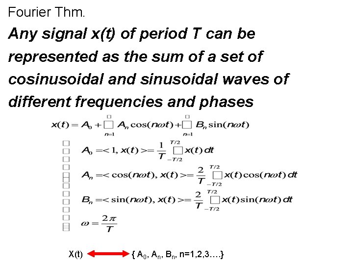
Fourier Thm. Any signal x(t) of period T can be represented as the sum of a set of cosinusoidal and sinusoidal waves of different frequencies and phases X(t) { A 0, An, Bn, n=1, 2, 3…. }

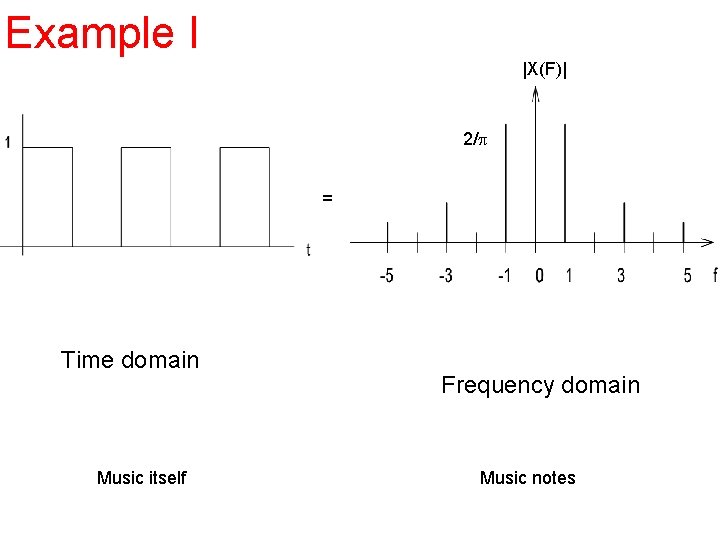
Example I |X(F)| 2/p = Time domain Music itself Frequency domain Music notes

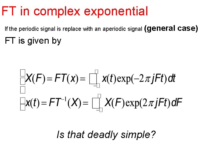
FT in complex exponential If the periodic signal is replace with an aperiodic signal (general FT is given by Is that deadly simple? case)

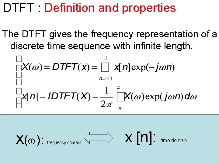
DTFT : Definition and properties The DTFT gives the frequency representation of a discrete time sequence with infinite length. X(w): frequency domain x [n]: time domain

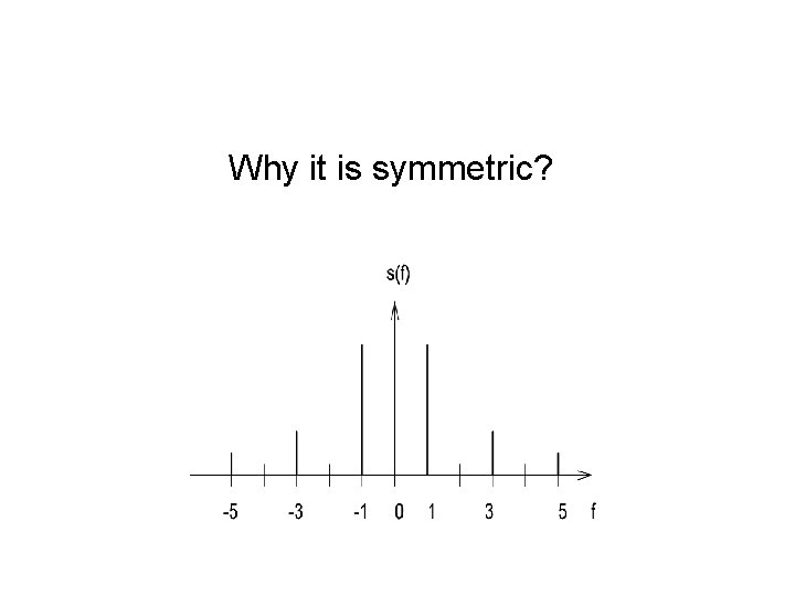
Why it is symmetric?

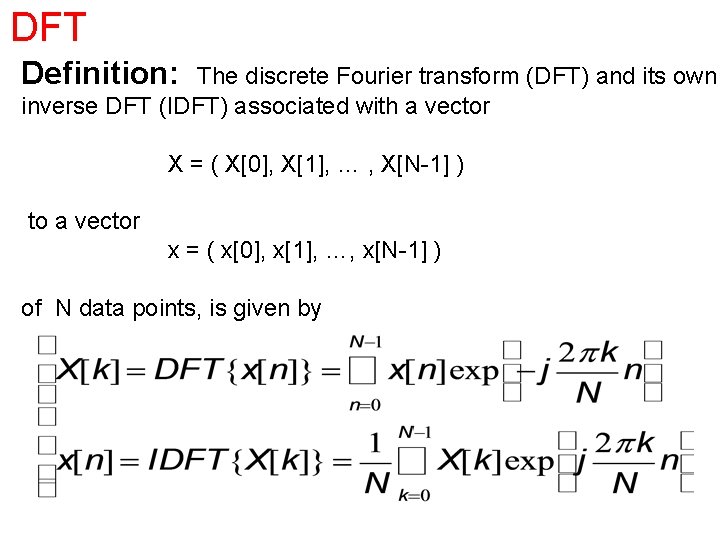
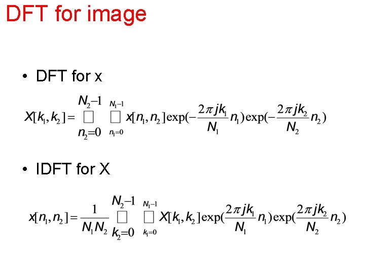
DFT Definition: The discrete Fourier transform (DFT) and its own inverse DFT (IDFT) associated with a vector X = ( X[0], X[1], … , X[N-1] ) to a vector x = ( x[0], x[1], …, x[N-1] ) of N data points, is given by

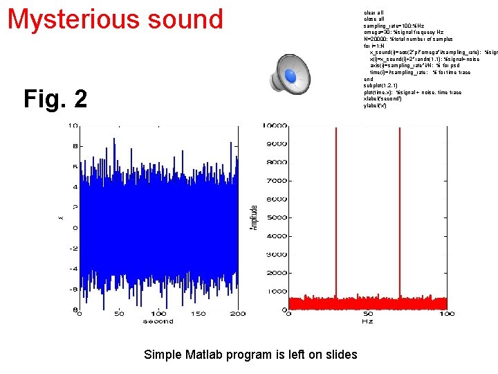
Mysterious sound Fig. 2 Simple Matlab program is left on slides clear all close all sampling_rate=100; %Hz omega=30; %signal frequecy Hz N=20000; %total number of samples for i=1: N x_sound(i)=cos(2*pi*omega*i/sampling_rate); %sign x(i)=x_sound(i)+2*randn(1, 1); %signal+noise axis(i)=sampling_rate*i/N; % for psd time(i)=i/sampling_rate; % for time trace end subplot(1, 2, 1) plot(time, x); %signal + noise, time trace xlabel('second') ylabel('x') subplot(1, 2, 2) plot(axis, abs(fft(x)), 'r'); % magnitude of signal xlabel('Hz'); ylabel('Amplitude') sound(x_sound)

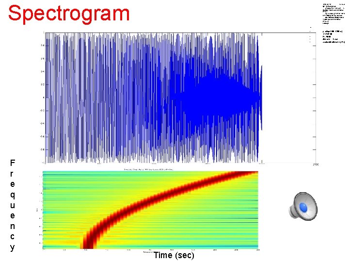
Spectrogram • • • t=0: 0. 001: 2; % 2 secs @ 1 k. Hz sample rate y=chirp(t, 100, 1, 200, 'q'); % Start @ 100 Hz, cross 200 Hz at t=1 sec spectrogram(y, 128, 120, 128, 1 E 3); % Display the spectrogram title('Quadratic Chirp: start at 100 Hz and cross 200 Hz at t=1 sec'); sound(y) • • • F r e q u e n c y Time (sec) y=chirp(t, 100, 1, 200, 'q'); % Start @ Fs=5000; filename = 'h. wav'; audiowrite(filename, y, Fs);

DFT for image • DFT for x • IDFT for X

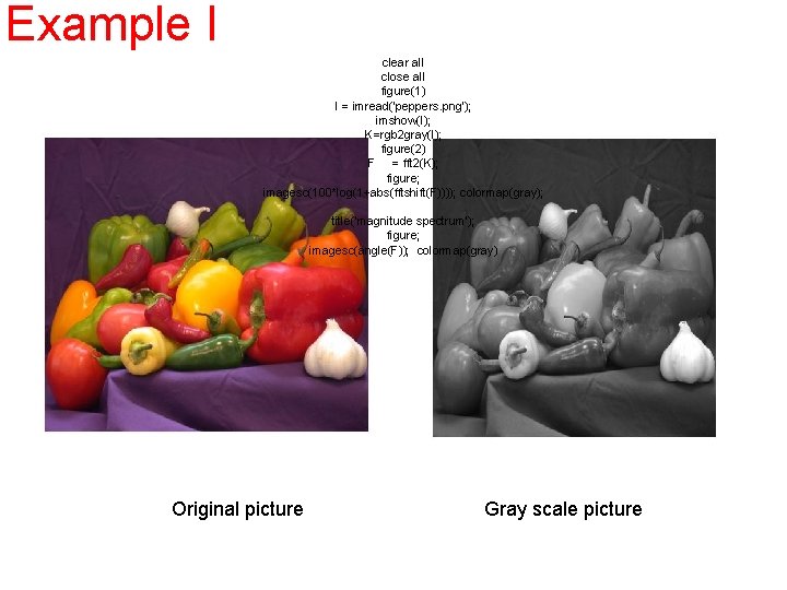
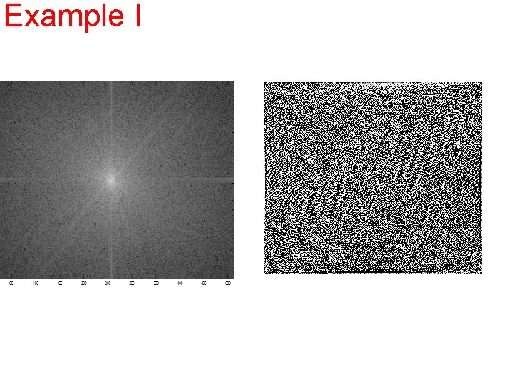
Example I clear all close all figure(1) I = imread('peppers. png'); imshow(I); K=rgb 2 gray(I); figure(2) F = fft 2(K); figure; imagesc(100*log(1+abs(fftshift(F)))); colormap(gray); title('magnitude spectrum'); figure; imagesc(angle(F)); colormap(gray) Original picture Gray scale picture

Example I

simple filter design • Notice two facts: • The signal has a frequency spectrum within the interval 0 to Fs/2 k. Hz. • The disturbance is at frequency F 0 (1. 5) k. Hz. • Design and implement a filter that rejects the disturbance without affecting the signal excessively. • We will follow three steps:

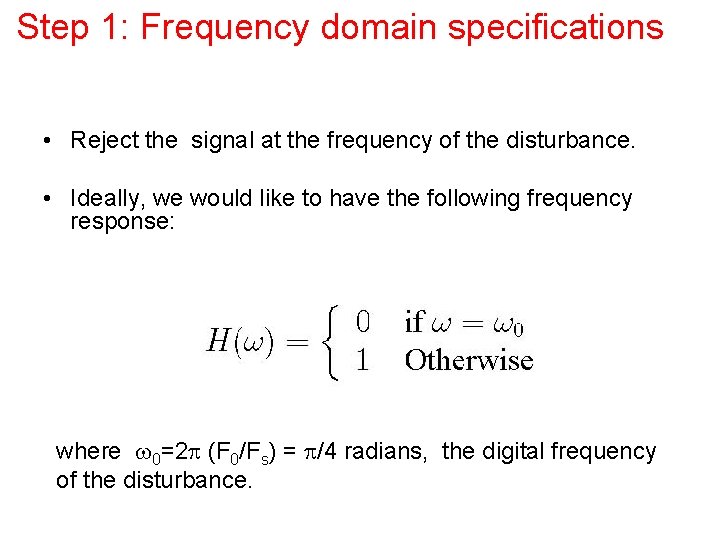
Step 1: Frequency domain specifications • Reject the signal at the frequency of the disturbance. • Ideally, we would like to have the following frequency response: where w 0=2 p (F 0/Fs) = p/4 radians, the digital frequency of the disturbance.

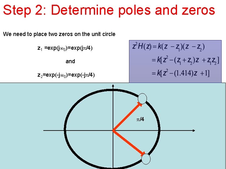
Step 2: Determine poles and zeros We need to place two zeros on the unit circle z 1 =exp(jw 0)=exp(jp/4) and z 2=exp(-jw 0)=exp(-jp/4) p/4

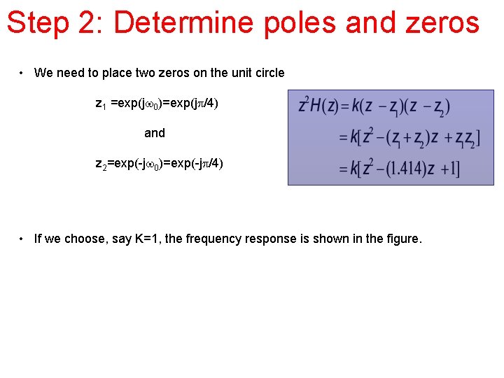
Step 2: Determine poles and zeros • We need to place two zeros on the unit circle z 1 =exp(jw 0)=exp(jp/4) and z 2=exp(-jw 0)=exp(-jp/4) • If we choose, say K=1, the frequency response is shown in the figure.

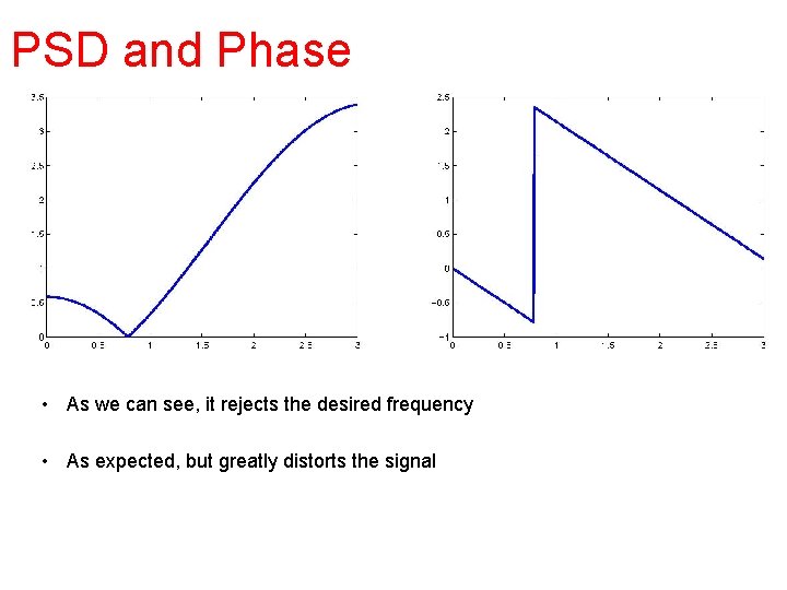
PSD and Phase • As we can see, it rejects the desired frequency • As expected, but greatly distorts the signal

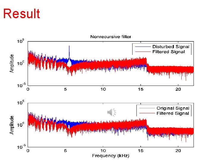
Result

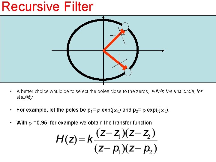
Recursive Filter • A better choice would be to select the poles close to the zeros, within the unit circle, for stability. • For example, let the poles be p 1= r exp(jw 0) and p 2= r exp(-jw 0). • With r =0. 95, for example we obtain the transfer function

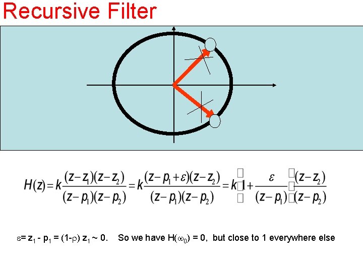
Recursive Filter e= z 1 - p 1 = (1 -r) z 1 ~ 0. So we have H(w 0) = 0, but close to 1 everywhere else

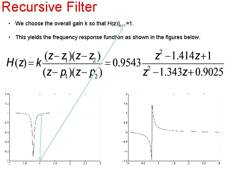
Recursive Filter • We choose the overall gain k so that H(z)|z=1=1. • This yields the frequency response function as shown in the figures below.

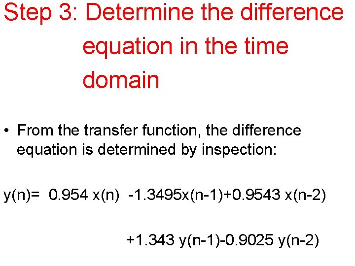
Step 3: Determine the difference equation in the time domain • From the transfer function, the difference equation is determined by inspection: y(n)= 0. 954 x(n) -1. 3495 x(n-1)+0. 9543 x(n-2) +1. 343 y(n-1)-0. 9025 y(n-2)

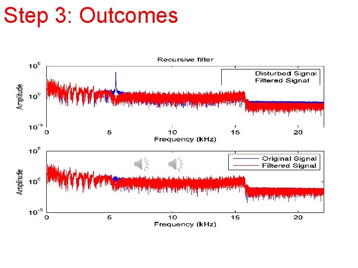
Step 3: difference equation • Easily implemented as a recursion in a high-level language. • The final signal y(n) with the frequency spectrum shown in the following Fig. , • We notice the absence of the disturbance.

Step 3: Outcomes

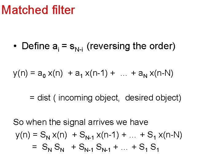
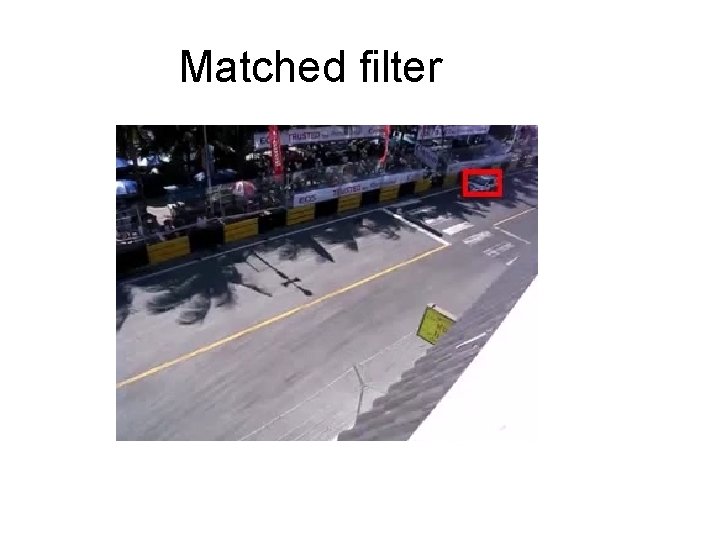
Matched filter • Define ai = s. N-i (reversing the order) y(n) = a 0 x(n) + a 1 x(n-1) + … + a. N x(n-N) = dist ( incoming object, desired object) So when the signal arrives we have y(n) = SN x(n) + SN-1 x(n-1) + … + S 1 x(n-N) = SN SN + SN-1 + … + S 1

Matched filter

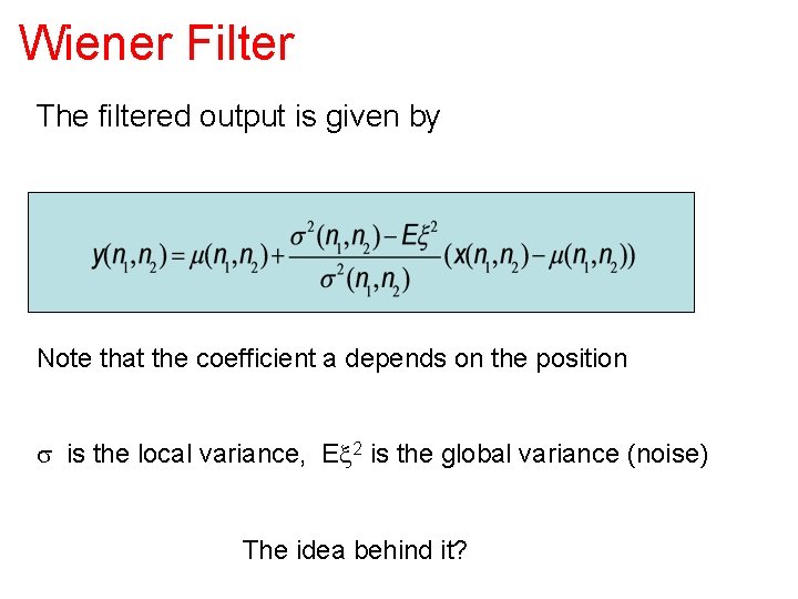
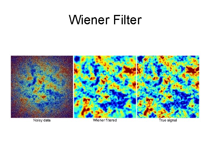
Wiener Filter The filtered output is given by Note that the coefficient a depends on the position s is the local variance, Ex 2 is the global variance (noise) The idea behind it?

Wiener Filter

past papers before the exam