DCSP16 Kalman Filter Jianfeng Feng Department of Computer

DCSP-16: Kalman Filter* Jianfeng Feng Department of Computer Science Warwick Univ. , UK Jianfeng@warwick. ac. uk http: //www. dcs. warwick. ac. uk/~feng/dcsp. html

Why we use Kalman Filter？ https: //www. youtube. com/watch? v=mwn 8 xhg. Np. FY

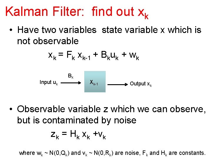
Kalman Filter: find out xk • Have two variables state variable x which is not observable xk = Fk xk-1 + Bkuk + wk Input uk Bk Xk-1 Output xk • Observable variable z which we can observe, but is contaminated by noise zk = Hk xk +vk where wk ~ N(0, Qk) and vk ~ N(0, Rk) are noise, Fk and Hk are constants.

Model https: //www. youtube. com/watch? v=4 Oer. Jm. Ppk. Rg

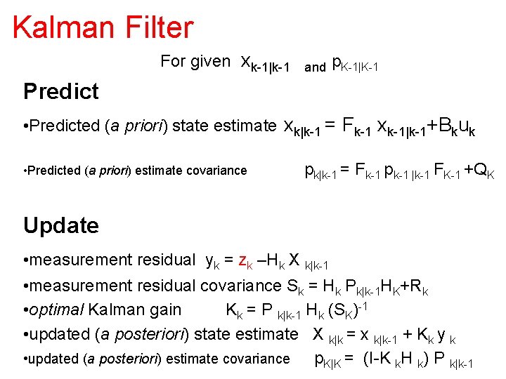
Kalman Filter For given xk-1|k-1 and p. K-1|K-1 Predict • Predicted (a priori) state estimate xk|k-1 = Fk-1 xk-1|k-1+Bkuk • Predicted (a priori) estimate covariance pk|k-1 = Fk-1 pk-1 |k-1 FK-1 +QK Update • measurement residual yk = zk –Hk X k|k-1 • measurement residual covariance Sk = Hk Pk|k-1 HK+Rk • optimal Kalman gain Kk = P k|k-1 Hk (SK)-1 • updated (a posteriori) state estimate X k|k = x k|k-1 + Kk y k • updated (a posteriori) estimate covariance p. K|K = (I-K k. H k) P k|k-1

Algorithm https: //www. youtube. com/watch? v=ul 3 u 2 y. LPw. U 0

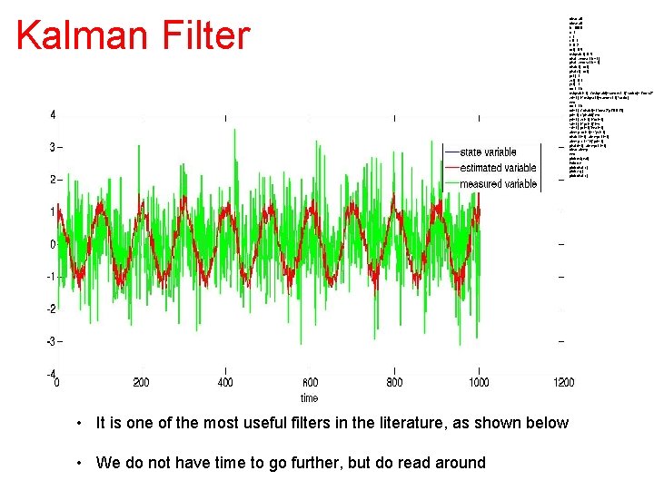
Kalman Filter • It is one of the most useful filters in the literature, as shown below • We do not have time to go further, but do read around clear all close all N=1000; q=1; r=1; f=0. 1; h=0. 2; x(1)=0. 5; xsignal(1)=0. 5; xhat=zeros(1, N+1); phat=zeros(1, N+1); xhat(1)=x(1); p(1)=1; z(1)=0. 1; y(1)=1; for i=1: N xsignal(i+1)=f*xsignal(i)+randn(1, 1)*sqrt(q)+1*cos(2*p z(i+1)=h*xsignal(i)+randn(1, 1)*sqrt(r); end for i=1: N x(i+1)=f*xhat(i)+1*cos(2*pi*0. 01*i); p(i+1)=f*phat(i)*f+q; y(i+1)=z(i+1)-h*x(i+1); s(i+1)=h*p(i+1)*h+r; k(i+1)=p(i+1)*h/s(i+1); atemp=x(i+1)+k*y(i+1); xhat(1, i+1)=atemp(1, i+1); atemp=(1 -k*h)*p(i+1); phat(i+1)=atemp(1, i+1); clear atemp end plot(xsignal); hold on plot(xhat, 'r') plot(z, 'g') plot(xhat, 'r')

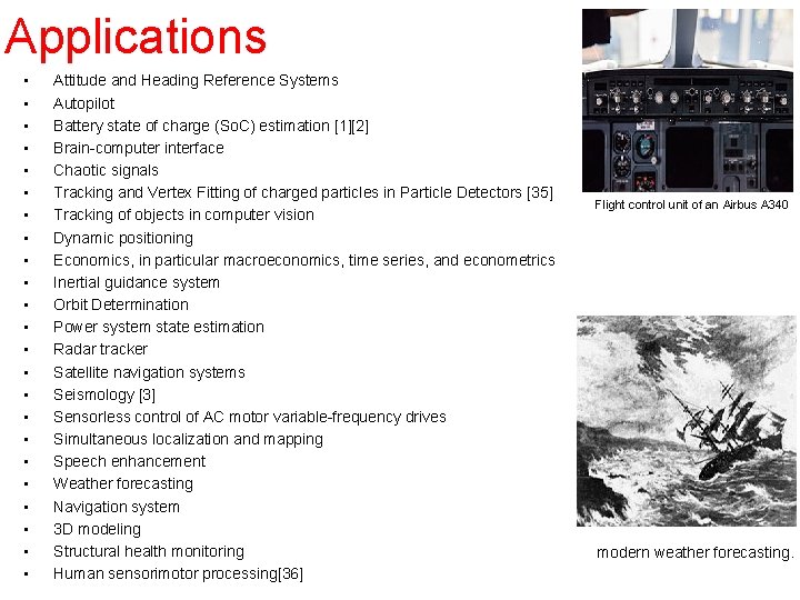
Applications • • • • • • Attitude and Heading Reference Systems Autopilot Battery state of charge (So. C) estimation [1][2] Brain-computer interface Chaotic signals Tracking and Vertex Fitting of charged particles in Particle Detectors [35] Tracking of objects in computer vision Dynamic positioning Economics, in particular macroeconomics, time series, and econometrics Inertial guidance system Orbit Determination Power system state estimation Radar tracker Satellite navigation systems Seismology [3] Sensorless control of AC motor variable-frequency drives Simultaneous localization and mapping Speech enhancement Weather forecasting Navigation system 3 D modeling Structural health monitoring Human sensorimotor processing[36] Flight control unit of an Airbus A 340 modern weather forecasting.

Next week • • • I will go through the materials we learnt this term In particular, possible questions in exam Hope to see you all here • • Will have a revision class next term Next week, hand in your assignment--no lecture (will let you know the time late on) Assignment deadline is next Thursday at noon