Data Warehousing and OLAP MIS 331 Chapter 5

Data Warehousing: and OLAP —MIS 331— — Chapter 5 — 2016/2017 Fall 1

Chapter 3: Data Warehousing and OLAP Technology for Data Mining n What is a data warehouse? n A multi-dimensional data model n Data warehouse architecture n Data warehouse implementation n Further development of data cube technology n From data warehousing to data mining 2

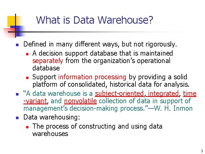
What is Data Warehouse? n n n Defined in many different ways, but not rigorously. n A decision support database that is maintained separately from the organization’s operational database n Support information processing by providing a solid platform of consolidated, historical data for analysis. “A data warehouse is a subject-oriented, integrated, time -variant, and nonvolatile collection of data in support of management’s decision-making process. ”—W. H. Inmon Data warehousing: n The process of constructing and using data warehouses 3

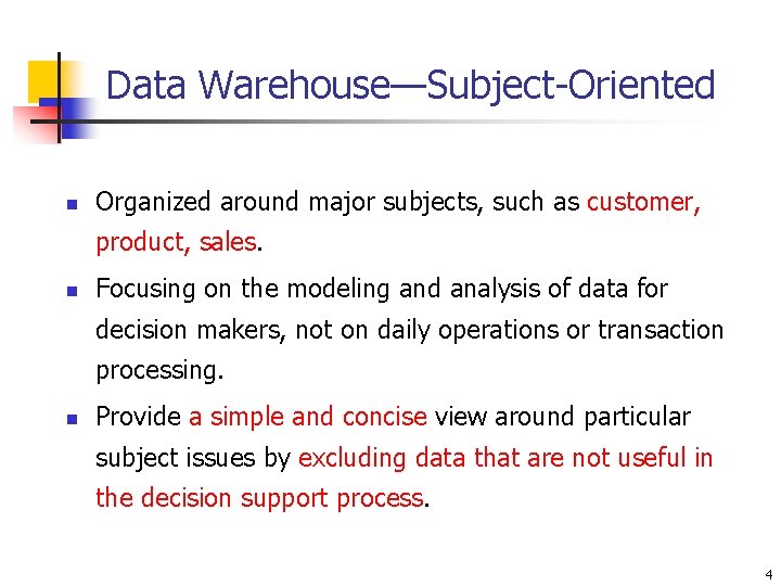
Data Warehouse—Subject-Oriented n Organized around major subjects, such as customer, product, sales. n Focusing on the modeling and analysis of data for decision makers, not on daily operations or transaction processing. n Provide a simple and concise view around particular subject issues by excluding data that are not useful in the decision support process. 4

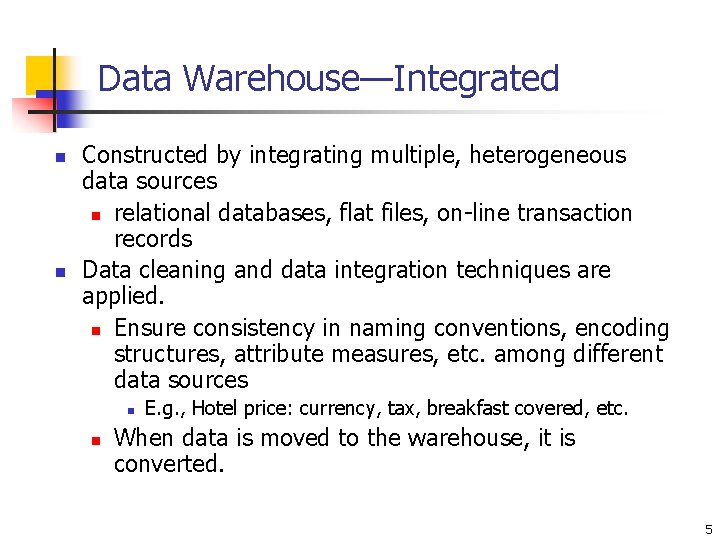
Data Warehouse—Integrated n n Constructed by integrating multiple, heterogeneous data sources n relational databases, flat files, on-line transaction records Data cleaning and data integration techniques are applied. n Ensure consistency in naming conventions, encoding structures, attribute measures, etc. among different data sources n n E. g. , Hotel price: currency, tax, breakfast covered, etc. When data is moved to the warehouse, it is converted. 5

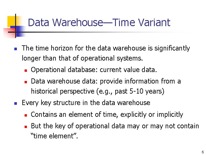
Data Warehouse—Time Variant n The time horizon for the data warehouse is significantly longer than that of operational systems. n n n Operational database: current value data. Data warehouse data: provide information from a historical perspective (e. g. , past 5 -10 years) Every key structure in the data warehouse n n Contains an element of time, explicitly or implicitly But the key of operational data may or may not contain “time element”. 6

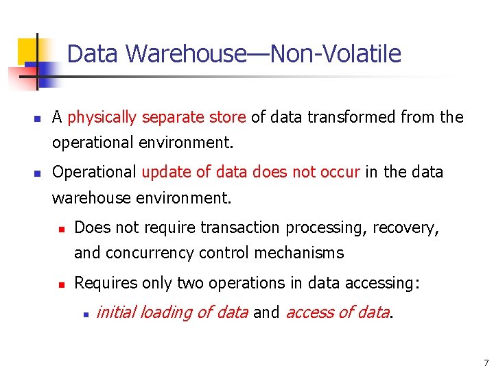
Data Warehouse—Non-Volatile n A physically separate store of data transformed from the operational environment. n Operational update of data does not occur in the data warehouse environment. n Does not require transaction processing, recovery, and concurrency control mechanisms n Requires only two operations in data accessing: n initial loading of data and access of data. 7

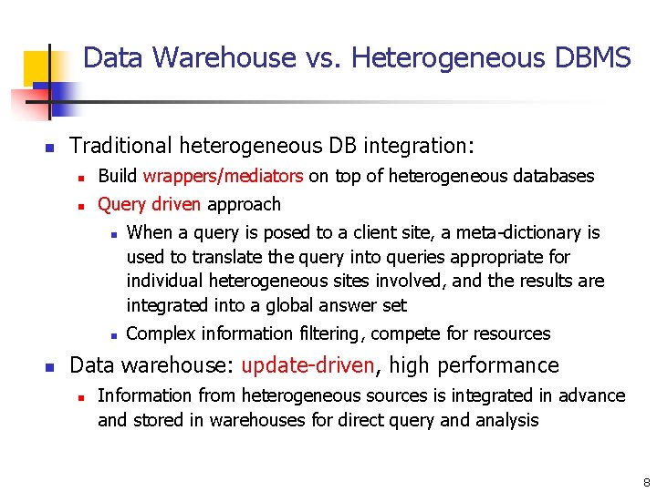
Data Warehouse vs. Heterogeneous DBMS n Traditional heterogeneous DB integration: n Build wrappers/mediators on top of heterogeneous databases n Query driven approach n n n When a query is posed to a client site, a meta-dictionary is used to translate the query into queries appropriate for individual heterogeneous sites involved, and the results are integrated into a global answer set Complex information filtering, compete for resources Data warehouse: update-driven, high performance n Information from heterogeneous sources is integrated in advance and stored in warehouses for direct query and analysis 8

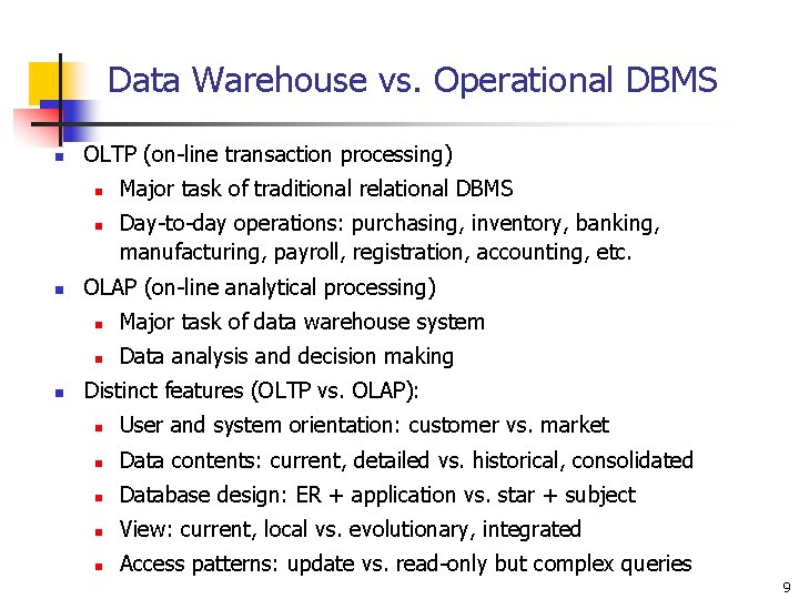
Data Warehouse vs. Operational DBMS n OLTP (on-line transaction processing) n n Major task of traditional relational DBMS Day-to-day operations: purchasing, inventory, banking, manufacturing, payroll, registration, accounting, etc. OLAP (on-line analytical processing) n Major task of data warehouse system n Data analysis and decision making Distinct features (OLTP vs. OLAP): n User and system orientation: customer vs. market n Data contents: current, detailed vs. historical, consolidated n Database design: ER + application vs. star + subject n View: current, local vs. evolutionary, integrated n Access patterns: update vs. read-only but complex queries 9

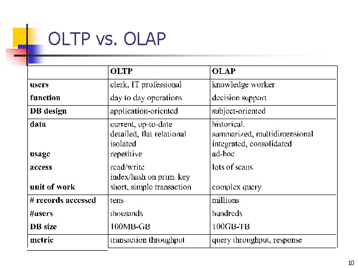
OLTP vs. OLAP 10

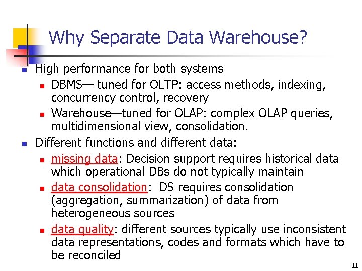
Why Separate Data Warehouse? n n High performance for both systems n DBMS— tuned for OLTP: access methods, indexing, concurrency control, recovery n Warehouse—tuned for OLAP: complex OLAP queries, multidimensional view, consolidation. Different functions and different data: n missing data: Decision support requires historical data which operational DBs do not typically maintain n data consolidation: DS requires consolidation (aggregation, summarization) of data from heterogeneous sources n data quality: different sources typically use inconsistent data representations, codes and formats which have to be reconciled 11

Chapter 2: Data Warehousing and OLAP Technology for Data Mining n What is a data warehouse? n A multi-dimensional data model n Data warehouse architecture n Data warehouse implementation n Further development of data cube technology n From data warehousing to data mining 12

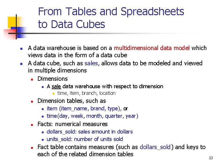
From Tables and Spreadsheets to Data Cubes n n A data warehouse is based on a multidimensional data model which views data in the form of a data cube A data cube, such as sales, allows data to be modeled and viewed in multiple dimensions n Dimensions n A sale data warehouse with respect to dimension n n Dimension tables, such as n n n item (item_name, brand, type), or time(day, week, month, quarter, year) Facts: numerical measures n n n time, item, branch, location dollars_sold: sales amount in dollars units_sold: number of units sold Fact table contains measures (such as dollars_sold) and keys to each of the related dimension tables 13

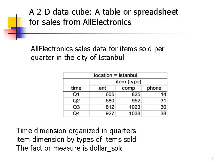
A 2 -D data cube: A table or spreadsheet for sales from All. Electronics sales data for items sold per quarter in the city of Istanbul Time dimension organized in quarters item dimension by types of items sold The fact or measure is dollar_sold 14

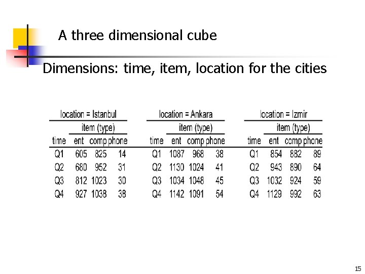
A three dimensional cube Dimensions: time, item, location for the cities 15

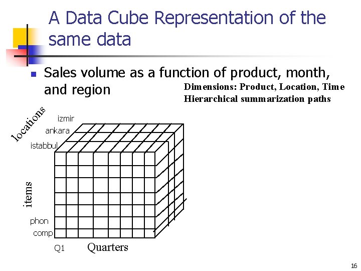
A Data Cube Representation of the same data n Sales volume as a function of product, month, Dimensions: Product, Location, Time and region izmir ankara istabbul items lo ca tio ns Hierarchical summarization paths phon comp Q 1 Quarters 16

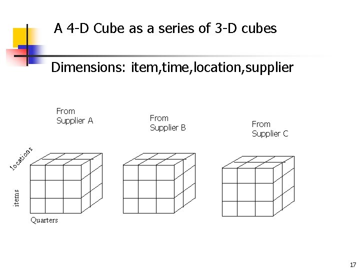
A 4 -D Cube as a series of 3 -D cubes Dimensions: item, time, location, supplier From Supplier B From Supplier C items lo ca tio ns From Supplier A Quarters 17

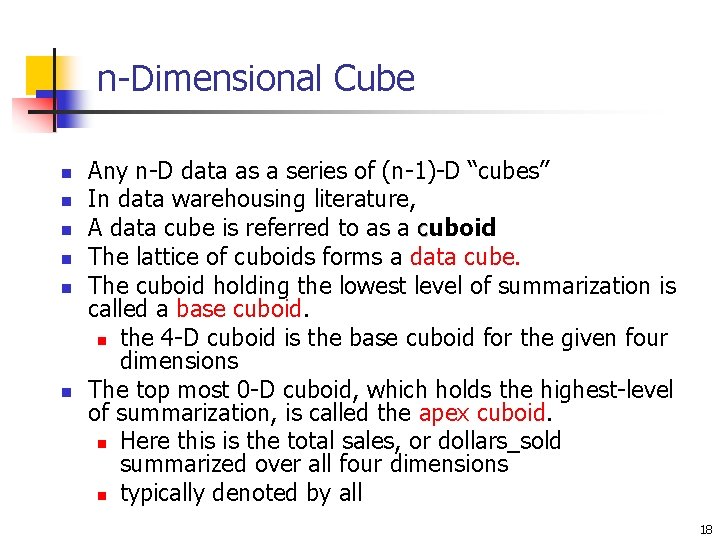
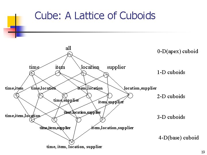
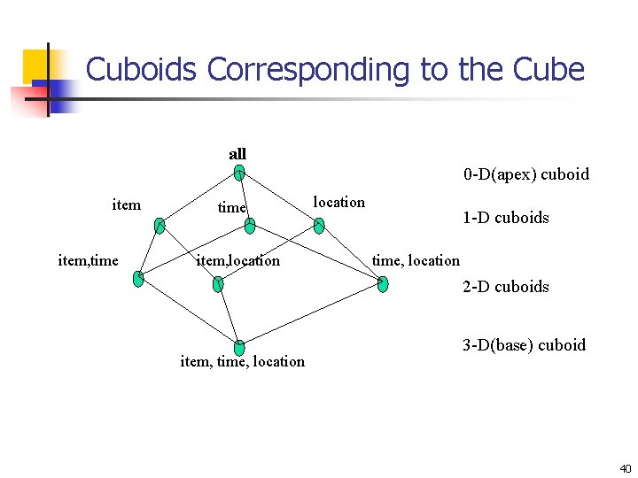
n-Dimensional Cube n n n Any n-D data as a series of (n-1)-D “cubes” In data warehousing literature, A data cube is referred to as a cuboid The lattice of cuboids forms a data cube. The cuboid holding the lowest level of summarization is called a base cuboid. n the 4 -D cuboid is the base cuboid for the given four dimensions The top most 0 -D cuboid, which holds the highest-level of summarization, is called the apex cuboid. n Here this is the total sales, or dollars_sold summarized over all four dimensions n typically denoted by all 18

Cube: A Lattice of Cuboids all time, item 0 -D(apex) cuboid item time, location item, location time, supplier time, item, location supplier location, supplier item, supplier time, location, supplier time, item, supplier 1 -D cuboids 2 -D cuboids 3 -D cuboids item, location, supplier 4 -D(base) cuboid time, item, location, supplier 19

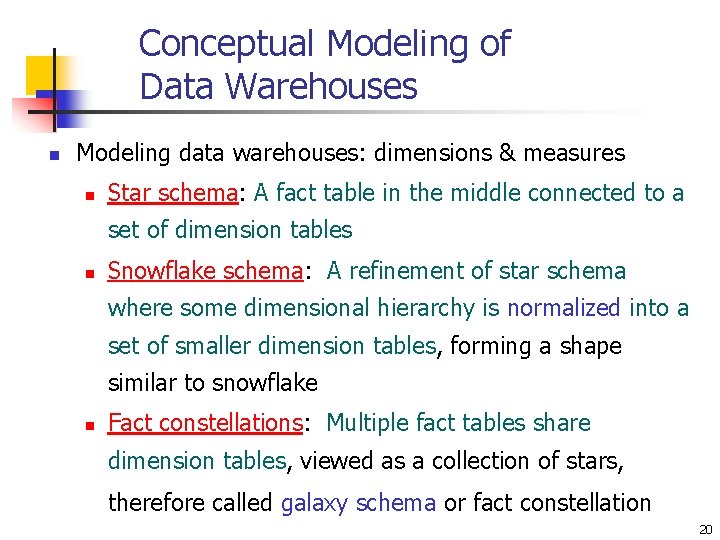
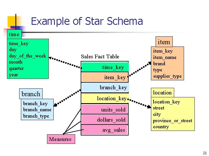
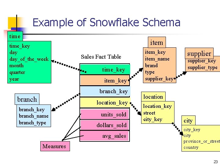
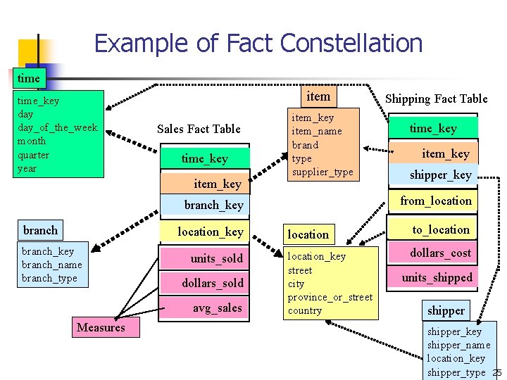
Conceptual Modeling of Data Warehouses n Modeling data warehouses: dimensions & measures n Star schema: A fact table in the middle connected to a set of dimension tables n Snowflake schema: A refinement of star schema where some dimensional hierarchy is normalized into a set of smaller dimension tables, forming a shape similar to snowflake n Fact constellations: Multiple fact tables share dimension tables, viewed as a collection of stars, therefore called galaxy schema or fact constellation 20

Example of Star Schema time item time_key day_of_the_week month quarter year Sales Fact Table time_key item_key branch_key branch_name branch_type location_key units_sold dollars_sold avg_sales item_key item_name brand type supplier_type location_key street city province_or_street country Measures 21

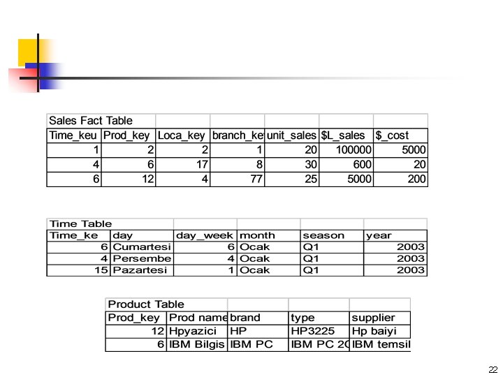
22

Example of Snowflake Schema time_key day_of_the_week month quarter year item Sales Fact Table time_key item_key branch location_key branch_name branch_type units_sold dollars_sold avg_sales Measures item_key item_name brand type supplier_key supplier_type location_key street city_key city province_or_street country 23

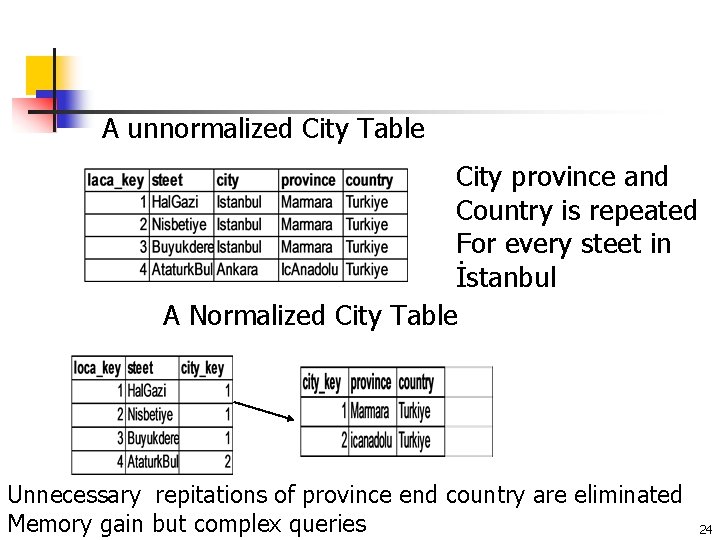
A unnormalized City Table City province and Country is repeated For every steet in İstanbul A Normalized City Table Unnecessary repitations of province end country are eliminated Memory gain but complex queries 24

Example of Fact Constellation time_key day_of_the_week month quarter year item Sales Fact Table time_key item_key item_name brand type supplier_type location_key branch_name branch_type units_sold dollars_sold avg_sales Measures time_key item_key shipper_key from_location branch_key branch Shipping Fact Table location to_location_key street city province_or_street country dollars_cost units_shipped shipper_key shipper_name location_key shipper_type 25

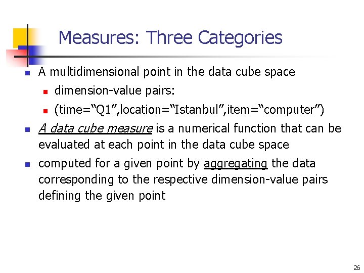
Measures: Three Categories n n A multidimensional point in the data cube space n dimension-value pairs: n (time=“Q 1”, location=“Istanbul”, item=“computer”) A data cube measure is a numerical function that can be evaluated at each point in the data cube space n computed for a given point by aggregating the data corresponding to the respective dimension-value pairs defining the given point 26

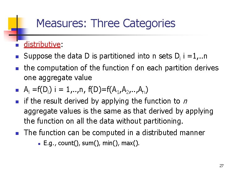
Measures: Three Categories n distributive: n Suppose the data D is partitioned into n sets Di i =1, . . n n n the computation of the function f on each partition derives one aggregate value Ai =f(Di) i = 1, . . , n, f(D)=f(A 1, A 2, . . , An) if the result derived by applying the function to n aggregate values is the same as that derived by applying the function on all the data without partitioning. The function can be computed in a distributed manner n E. g. , count(), sum(), min(), max(). 27

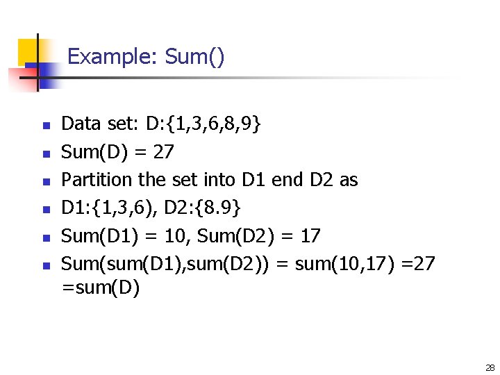
Example: Sum() n n n Data set: D: {1, 3, 6, 8, 9} Sum(D) = 27 Partition the set into D 1 end D 2 as D 1: {1, 3, 6), D 2: {8. 9} Sum(D 1) = 10, Sum(D 2) = 17 Sum(sum(D 1), sum(D 2)) = sum(10, 17) =27 =sum(D) 28

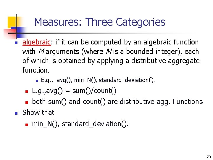
Measures: Three Categories n algebraic: if it can be computed by an algebraic function with M arguments (where M is a bounded integer), each of which is obtained by applying a distributive aggregate function. n n E. g. , avg(), min_N(), standard_deviation(). n E. g. , avg() = sum()/count() n both sum() and count() are distributive agg. Functions Show that n min_N(), standard_deviation(). 29

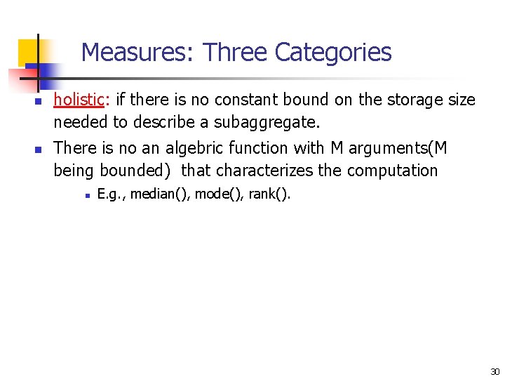
Measures: Three Categories n n holistic: if there is no constant bound on the storage size needed to describe a subaggregate. There is no an algebric function with M arguments(M being bounded) that characterizes the computation n E. g. , median(), mode(), rank(). 30

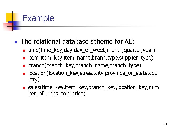
Example n The relational database scheme for AE: n n n time(time_key, day_of_week, month, quarter, year) item(item_key, item_name, brand, type, supplier_type) branch(branch_key, branch_name, branch_type) location(location_key, street, city, province_or_state, cou ntry) sales(time_key, item_key, branch_key, location_key, num ber_of_units_sold, price) 31

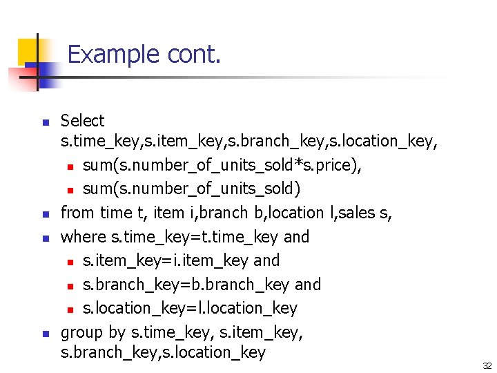
Example cont. n n Select s. time_key, s. item_key, s. branch_key, s. location_key, n sum(s. number_of_units_sold*s. price), n sum(s. number_of_units_sold) from time t, item i, branch b, location l, sales s, where s. time_key=t. time_key and n s. item_key=i. item_key and n s. branch_key=b. branch_key and n s. location_key=l. location_key group by s. time_key, s. item_key, s. branch_key, s. location_key 32

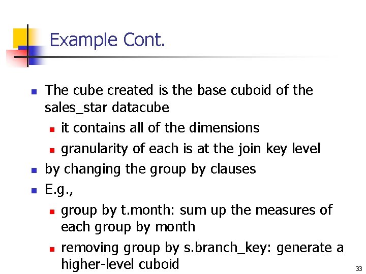
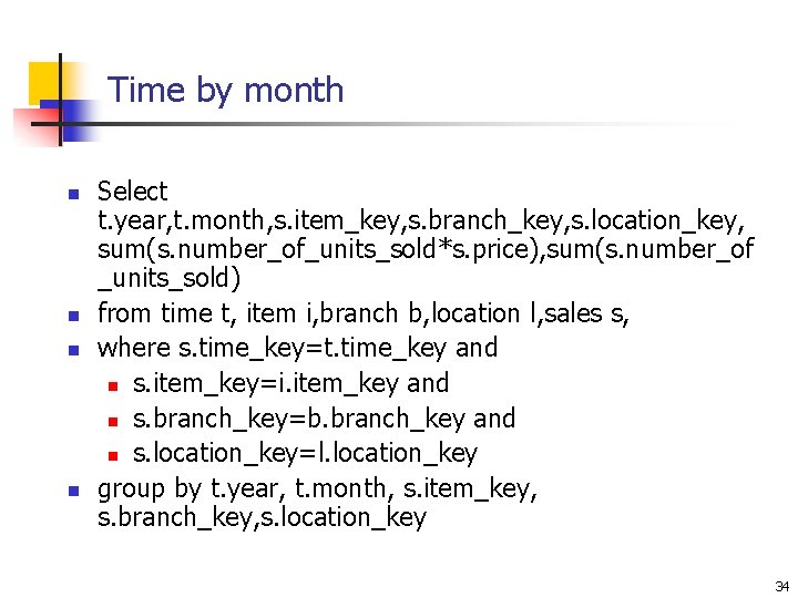
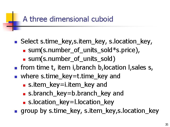
Example Cont. n n n The cube created is the base cuboid of the sales_star datacube n it contains all of the dimensions n granularity of each is at the join key level by changing the group by clauses E. g. , n group by t. month: sum up the measures of each group by month n removing group by s. branch_key: generate a higher-level cuboid 33

Time by month n n Select t. year, t. month, s. item_key, s. branch_key, s. location_key, sum(s. number_of_units_sold*s. price), sum(s. number_of _units_sold) from time t, item i, branch b, location l, sales s, where s. time_key=t. time_key and n s. item_key=i. item_key and n s. branch_key=b. branch_key and n s. location_key=l. location_key group by t. year, t. month, s. item_key, s. branch_key, s. location_key 34

A three dimensional cuboid n n Select s. time_key, s. item_key, s. location_key, n sum(s. number_of_units_sold*s. price), n sum(s. number_of_units_sold) from time t, item i, branch b, location l, sales s, where s. time_key=t. time_key and n s. item_key=i. item_key and n s. branch_key=b. branch_key and n s. location_key=l. location_key group by s. time_key, s. item_key, s. location_key 35

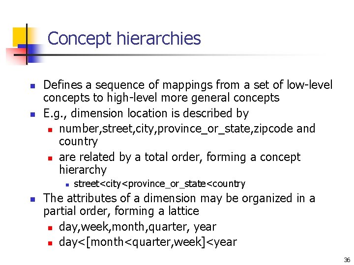
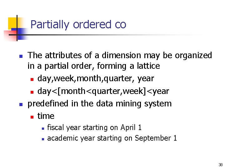
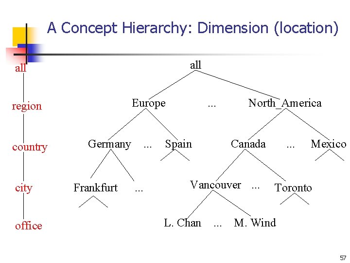
Concept hierarchies n n Defines a sequence of mappings from a set of low-level concepts to high-level more general concepts E. g. , dimension location is described by n number, street, city, province_or_state, zipcode and country n are related by a total order, forming a concept hierarchy n n street<city<province_or_state<country The attributes of a dimension may be organized in a partial order, forming a lattice n day, week, month, quarter, year n day<[month<quarter, week]<year 36

A Concept Hierarchy: Dimension (location) all Europe region country city office Germany Frankfurt . . Spain North_America Canada Vancouver. . . L. Chan . . . Mexico Toronto M. Wind 37

Partially ordered co n n The attributes of a dimension may be organized in a partial order, forming a lattice n day, week, month, quarter, year n day<[month<quarter, week]<year predefined in the data mining system n time n n fiscal year starting on April 1 academic year starting on September 1 38

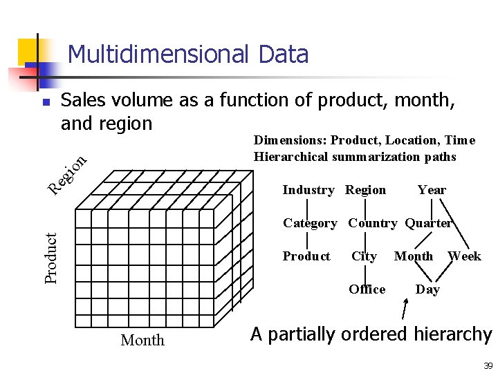
Multidimensional Data Sales volume as a function of product, month, and region Dimensions: Product, Location, Time Hierarchical summarization paths gi on n Re Industry Region Year Product Category Country Quarter Product City Office Month Week Day A partially ordered hierarchy 39

Cuboids Corresponding to the Cube all 0 -D(apex) cuboid item, time item, location 1 -D cuboids time, location 2 -D cuboids item, time, location 3 -D(base) cuboid 40

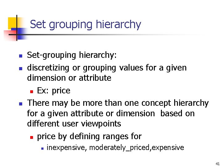
Set grouping hierarchy n n n Set-grouping hierarchy: discretizing or grouping values for a given dimension or attribute n Ex: price There may be more than one concept hierarchy for a given attribute or dimension based on different user viewpoints n price by defining ranges for n inexpensive, moderately_priced, expensive 41

How defined? n n provided by manually by n system users n domain experts n knowledge engineers or automatically generated based on statistical analysis of the data distribution 42

Typical OLAP Operations n n n In the multidimensional model data are organized into multiple dimensions each dimension contains multiple levels of abstraction defined by concept hierarchies This organization provides users with the flexibility to view data from different perspectives 43

Example n n n Refer to figure 2. 10 in Han’s book data cube for All. Ells sales n dimensions: location, time, item n location -- city n time -- quarters n item -- item types measure displayed is dollars-sold 44

Cuboids Corresponding to the Cube all 0 -D(apex) cuboid item, time item, location 1 -D cuboids time, location 2 -D cuboids item, time, location 3 -D(base) cuboid 45

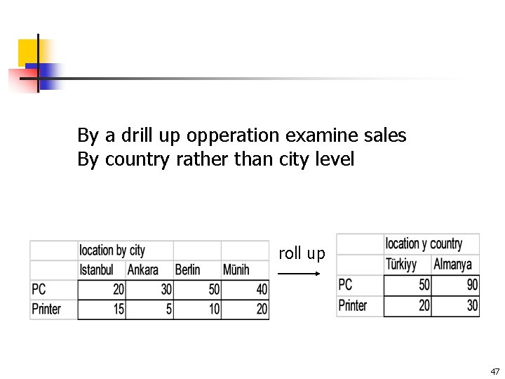
Roll-up (drill-up) n Climbing up a concept hierarchy for a dimension or n by dimension reduction n Ex: roll-up operation aggregates data by ascending the location hierarchy n from the level of city n to the level of country n rather than grouping the data by city, the cubes n groups the data by country 46

By a drill up opperation examine sales By country rather than city level roll up 47

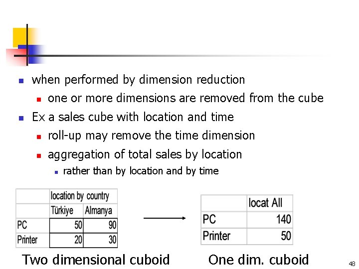
n when performed by dimension reduction n n one or more dimensions are removed from the cube Ex a sales cube with location and time n roll-up may remove the time dimension n aggregation of total sales by location n rather than by location and by time Two dimensional cuboid One dim. cuboid 48

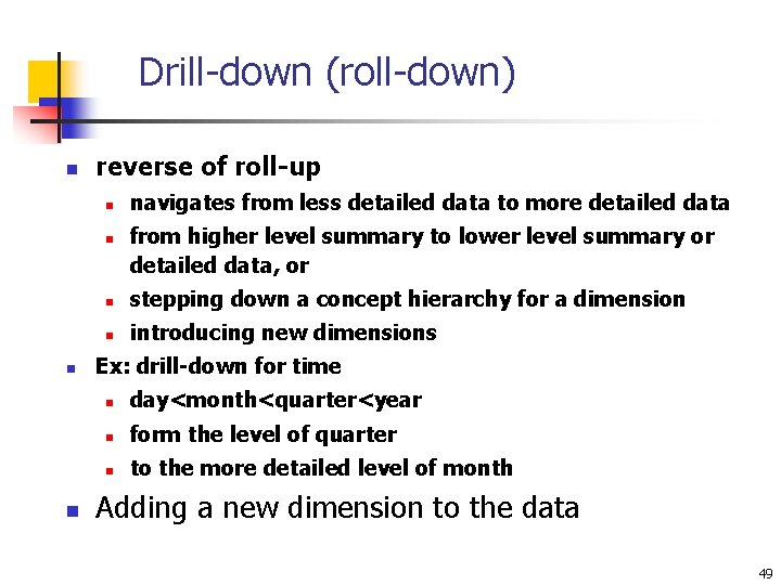
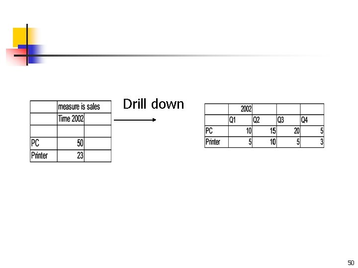
Drill-down (roll-down) n reverse of roll-up n n navigates from less detailed data to more detailed data from higher level summary to lower level summary or detailed data, or n stepping down a concept hierarchy for a dimension n introducing new dimensions Ex: drill-down for time n day<month<quarter<year n form the level of quarter n to the more detailed level of month Adding a new dimension to the data 49

Drill down 50

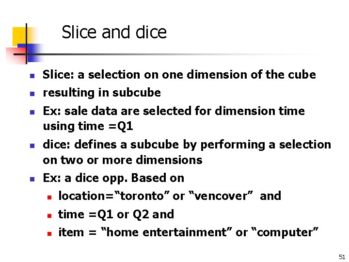
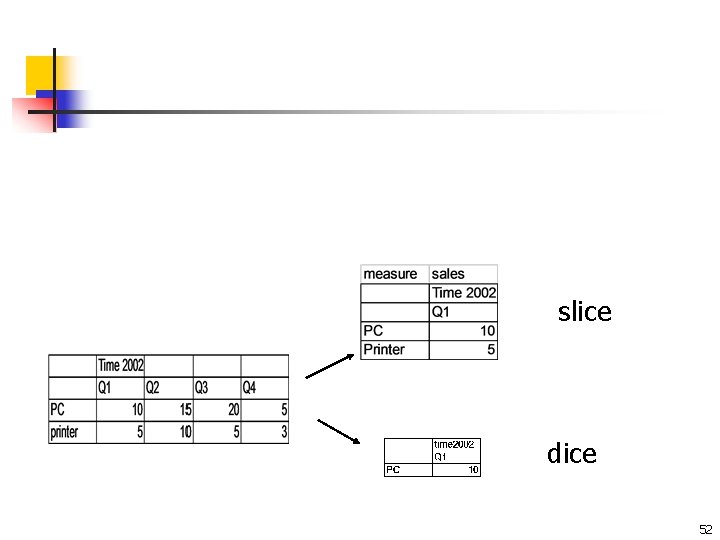
Slice and dice n Slice: a selection on one dimension of the cube n resulting in subcube n n n Ex: sale data are selected for dimension time using time =Q 1 dice: defines a subcube by performing a selection on two or more dimensions Ex: a dice opp. Based on n location=“toronto” or “vencover” and n time =Q 1 or Q 2 and n item = “home entertainment” or “computer” 51

slice dice 52

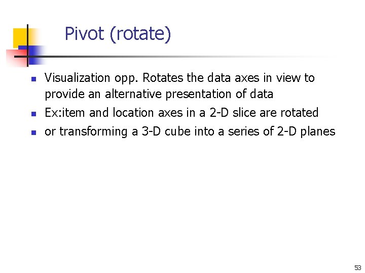
Pivot (rotate) n Visualization opp. Rotates the data axes in view to provide an alternative presentation of data n Ex: item and location axes in a 2 -D slice are rotated n or transforming a 3 -D cube into a series of 2 -D planes 53

Other OLAP operations n n drill across: involving (across) more than one fact table drill through: through the bottom level of the cube to its back-end relational tables (using SQL) n ranking the top N or bottom N items in lists n moving averages n growth rates n interests 54

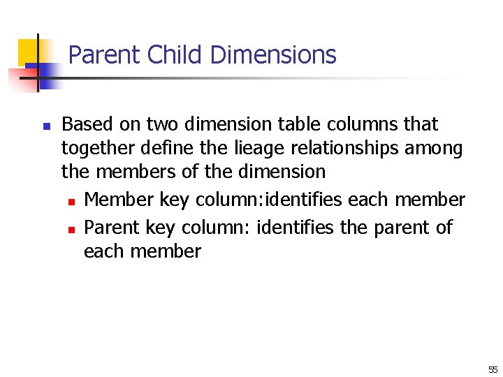
Parent Child Dimensions n Based on two dimension table columns that together define the lieage relationships among the members of the dimension n Member key column: identifies each member n Parent key column: identifies the parent of each member 55

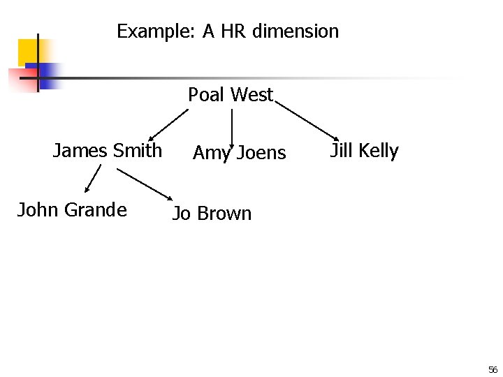
Example: A HR dimension Poal West James Smith John Grande Amy Joens Jill Kelly Jo Brown 56

A Concept Hierarchy: Dimension (location) all Europe region country city office Germany Frankfurt . . Spain North_America Canada Vancouver. . . L. Chan . . . Mexico Toronto M. Wind 57

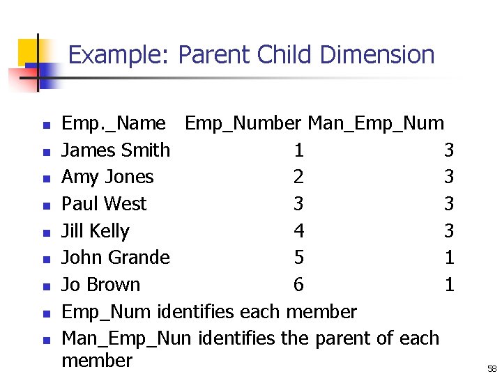
Example: Parent Child Dimension n n n n Emp. _Name Emp_Number Man_Emp_Num James Smith 1 3 Amy Jones 2 3 Paul West 3 3 Jill Kelly 4 3 John Grande 5 1 Jo Brown 6 1 Emp_Num identifies each member Man_Emp_Nun identifies the parent of each member 58

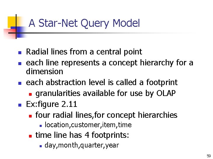
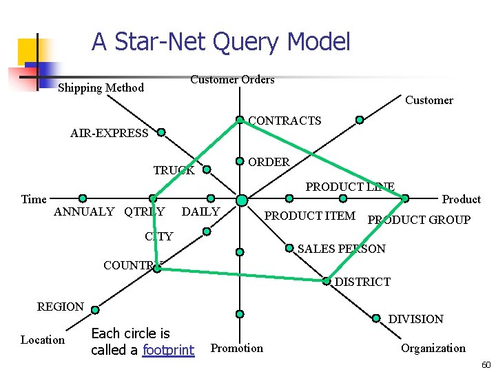
A Star-Net Query Model n n Radial lines from a central point each line represents a concept hierarchy for a dimension each abstraction level is called a footprint n granularities available for use by OLAP Ex: figure 2. 11 n four radial lines, for concept hierarchies n n location, customer, item, time line has 4 footprints: n day, month, quarter, year 59

A Star-Net Query Model Customer Orders Shipping Method Customer CONTRACTS AIR-EXPRESS ORDER TRUCK Time PRODUCT LINE ANNUALY QTRLY DAILY CITY Product PRODUCT ITEM PRODUCT GROUP SALES PERSON COUNTRY DISTRICT REGION Location Each circle is called a footprint DIVISION Promotion Organization 60

Chapter 2: Data Warehousing and OLAP Technology for Data Mining n What is a data warehouse? n A multi-dimensional data model n Data warehouse architecture n Data warehouse implementation n Further development of data cube technology n From data warehousing to data mining 61

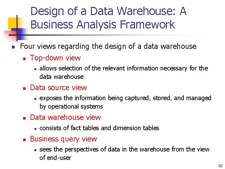
Design of a Data Warehouse: A Business Analysis Framework n Four views regarding the design of a data warehouse n Top-down view n n Data source view n n exposes the information being captured, stored, and managed by operational systems Data warehouse view n n allows selection of the relevant information necessary for the data warehouse consists of fact tables and dimension tables Business query view n sees the perspectives of data in the warehouse from the view of end-user 62

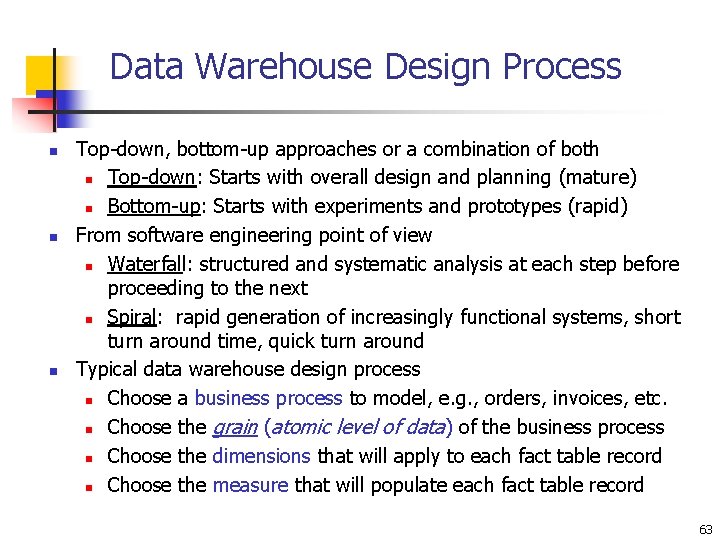
Data Warehouse Design Process n n n Top-down, bottom-up approaches or a combination of both n Top-down: Starts with overall design and planning (mature) n Bottom-up: Starts with experiments and prototypes (rapid) From software engineering point of view n Waterfall: structured and systematic analysis at each step before proceeding to the next n Spiral: rapid generation of increasingly functional systems, short turn around time, quick turn around Typical data warehouse design process n Choose a business process to model, e. g. , orders, invoices, etc. n Choose the grain (atomic level of data) of the business process n Choose the dimensions that will apply to each fact table record n Choose the measure that will populate each fact table record 63

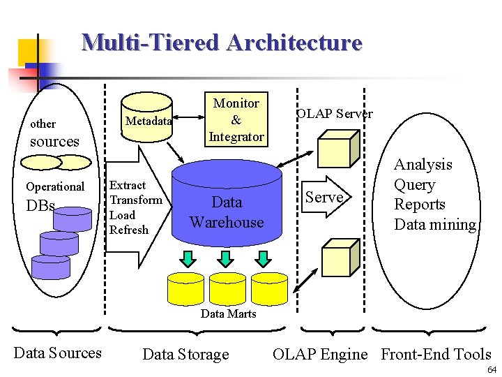
Multi-Tiered Architecture other Metadata sources Operational DBs Extract Transform Load Refresh Monitor & Integrator Data Warehouse OLAP Server Serve Analysis Query Reports Data mining Data Marts Data Sources Data Storage OLAP Engine Front-End Tools 64

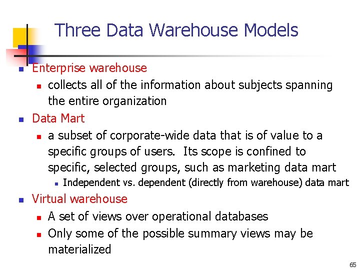
Three Data Warehouse Models n n Enterprise warehouse n collects all of the information about subjects spanning the entire organization Data Mart n a subset of corporate-wide data that is of value to a specific groups of users. Its scope is confined to specific, selected groups, such as marketing data mart n n Independent vs. dependent (directly from warehouse) data mart Virtual warehouse n A set of views over operational databases n Only some of the possible summary views may be materialized 65

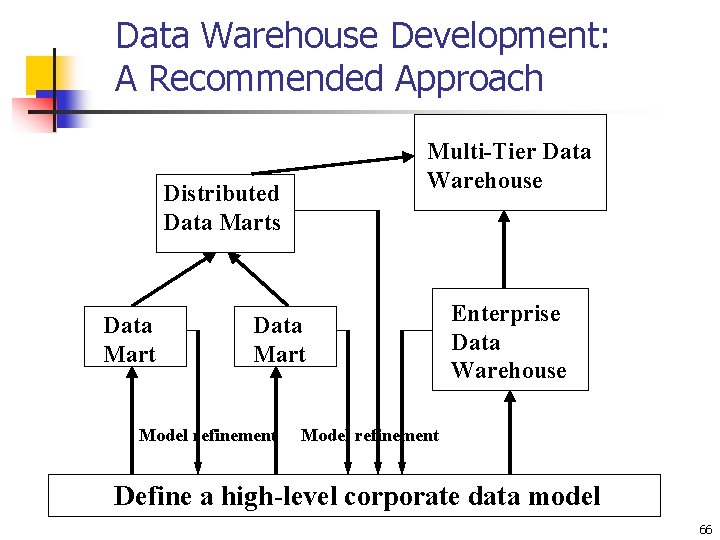
Data Warehouse Development: A Recommended Approach Multi-Tier Data Warehouse Distributed Data Marts Data Mart Model refinement Enterprise Data Warehouse Model refinement Define a high-level corporate data model 66

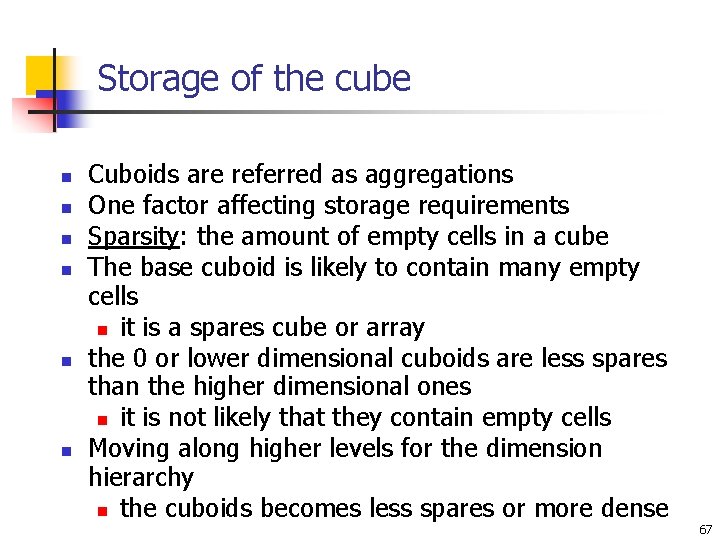
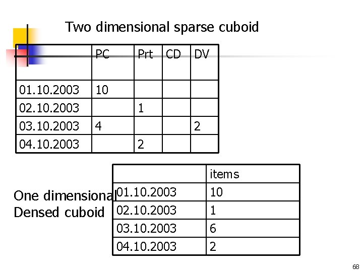
Storage of the cube n n n Cuboids are referred as aggregations One factor affecting storage requirements Sparsity: the amount of empty cells in a cube The base cuboid is likely to contain many empty cells n it is a spares cube or array the 0 or lower dimensional cuboids are less spares than the higher dimensional ones n it is not likely that they contain empty cells Moving along higher levels for the dimension hierarchy n the cuboids becomes less spares or more dense 67

Two dimensional sparse cuboid PC 01. 10. 2003 02. 10. 2003 10 03. 10. 2003 04. 10. 2003 4 Prt CD DV 1 2 2 03. 10. 2003 items 10 1 6 04. 10. 2003 2 One dimensional 01. 10. 2003 Densed cuboid 02. 10. 2003 68

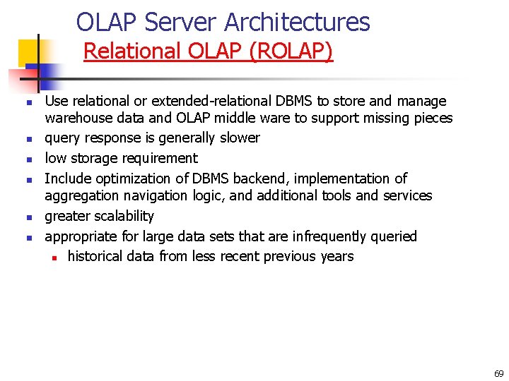
OLAP Server Architectures Relational OLAP (ROLAP) n n n Use relational or extended-relational DBMS to store and manage warehouse data and OLAP middle ware to support missing pieces query response is generally slower low storage requirement Include optimization of DBMS backend, implementation of aggregation navigation logic, and additional tools and services greater scalability appropriate for large data sets that are infrequently queried n historical data from less recent previous years 69

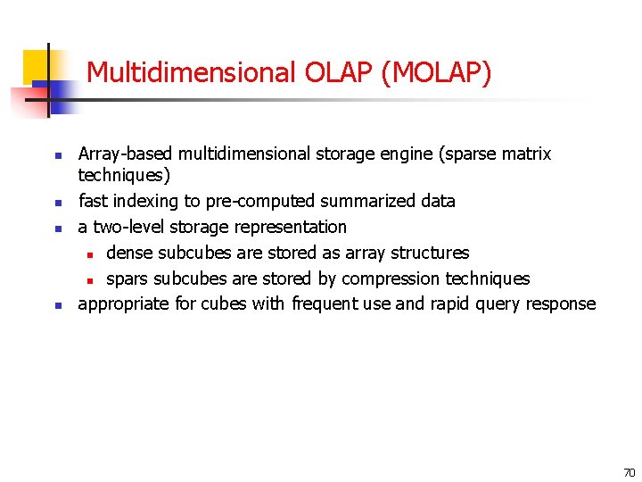
Multidimensional OLAP (MOLAP) n n Array-based multidimensional storage engine (sparse matrix techniques) fast indexing to pre-computed summarized data a two-level storage representation n dense subcubes are stored as array structures n spars subcubes are stored by compression techniques appropriate for cubes with frequent use and rapid query response 70

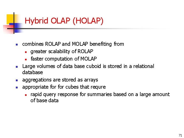
Hybrid OLAP (HOLAP) n n combines ROLAP and MOLAP benefiting from n greater scalability of ROLAP n faster computation of MOLAP Large volumes of data base cuboid is stored in a relational database aggregations are stored as arrays appropriate for cubes that requre n rapid query response for summaries based on a large amount of base data 71

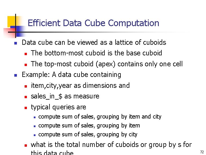
Efficient Data Cube Computation n n Data cube can be viewed as a lattice of cuboids n The bottom-most cuboid is the base cuboid n The top-most cuboid (apex) contains only one cell Example: A data cube containing n item, city, year as dimensions and n sales_in_$ as measure n typical queries are n n compute sum of sales, grouping by item and city n compute sum of sales, grouping by item n compute sum of sales, grouping by city what is the total number of cuboids or group by s for 72

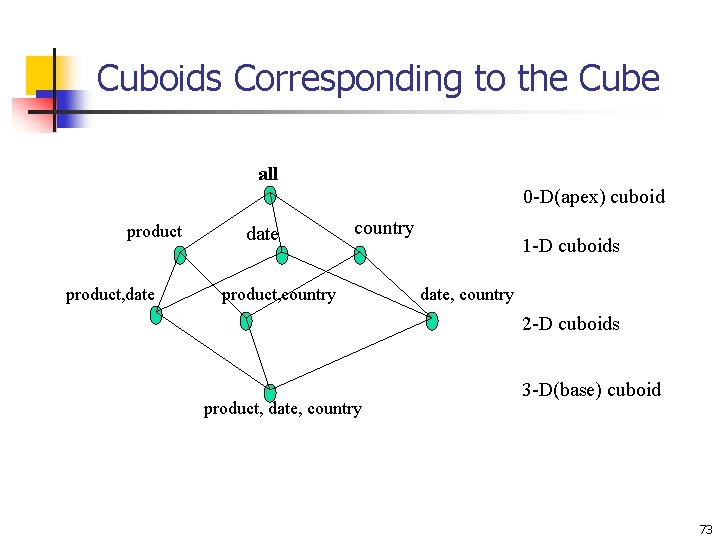
Cuboids Corresponding to the Cube all 0 -D(apex) cuboid product, date country product, country 1 -D cuboids date, country 2 -D cuboids product, date, country 3 -D(base) cuboid 73

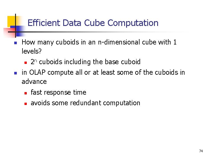
Efficient Data Cube Computation n How many cuboids in an n-dimensional cube with 1 levels? n n 2 n cuboids including the base cuboid in OLAP compute all or at least some of the cuboids in advance n fast response time n avoids some redundant computation 74

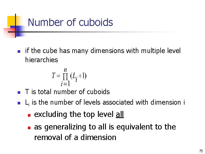
Number of cuboids n if the cube has many dimensions with multiple level hierarchies n T is total number of cuboids n Li is the number of levels associated with dimension i n n excluding the top level all as generalizing to all is equivalent to the removal of a dimension 75

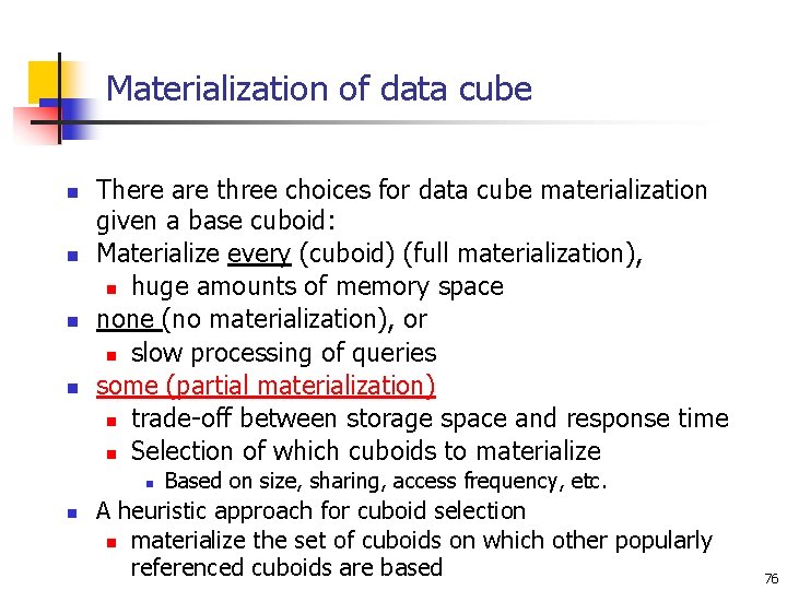
Materialization of data cube n n There are three choices for data cube materialization given a base cuboid: Materialize every (cuboid) (full materialization), n huge amounts of memory space none (no materialization), or n slow processing of queries some (partial materialization) n trade-off between storage space and response time n Selection of which cuboids to materialize n n Based on size, sharing, access frequency, etc. A heuristic approach for cuboid selection n materialize the set of cuboids on which other popularly referenced cuboids are based 76

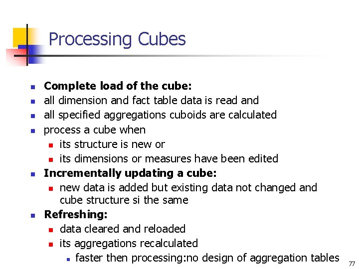
Processing Cubes n n n Complete load of the cube: all dimension and fact table data is read and all specified aggregations cuboids are calculated process a cube when n its structure is new or n its dimensions or measures have been edited Incrementally updating a cube: n new data is added but existing data not changed and cube structure si the same Refreshing: n data cleared and reloaded n its aggregations recalculated n faster then processing: no design of aggregation tables 77

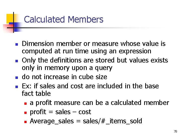
Calculated Members n n Dimension member or measure whose value is computed at run time using an expression Only the definitions are stored but values exists only in memory upon a query do not increase in cube size Ex: if sales and cost are included in the base fact table n a profit measure can be a calculated member n profit = sales – cost n Average_sales = sales/#_items_sold 78

Virtual cubes n n n Combination of multiple cubes in one logical cube n can be based on a single cube to expose only selected subsets of measures and dimensions Require no physical space n store only the dimensions information not actual data provide a valuable security functiton n limiting the access of some users 79

Member Properties n n Attribute of a dimension member provides additional information about the member a column in the same dimension table as the associated members used in queries n provide users more options when analysing cube data 80

Example: time table n n A typical time table: (time_id, day, month, quarter, year, business day, leap, day of the week) n dimension levels day<month<quarter<year n member properties for day: n weekend or business day: 0 or 1 n day of the week: 1, 2, 3, . . . , 7 n a member property for year is n whether it is leap year or not: 0 or 1 81

Virtual Dimensions n n Logical dimension based on a member property of a level in a physical dimension enables users to analyze cube data based on the member properties of dimension levels add a virtual dimension to a cube only if n the dimension that supplies its member property is also included in the cube adding a virtual dimension does not increase cube size n not affect cube processing time n n calculated in memory when needed query processing time is slower 82

Example n n The business day column was a member property for day level of the time dimension the user may want to investigate sales by type of day (business or weekend) makes business day member property as a virtual dimension of the sale cube 83

Exercise n How do you represent the same organizational chart by treditional concept hyerarchies? 84

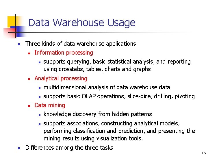
Data Warehouse Usage n Three kinds of data warehouse applications n Information processing n n n Analytical processing n multidimensional analysis of data warehouse data n supports basic OLAP operations, slice-dice, drilling, pivoting Data mining n n n supports querying, basic statistical analysis, and reporting using crosstabs, tables, charts and graphs knowledge discovery from hidden patterns supports associations, constructing analytical models, performing classification and prediction, and presenting the mining results using visualization tools. Differences among the three tasks 85

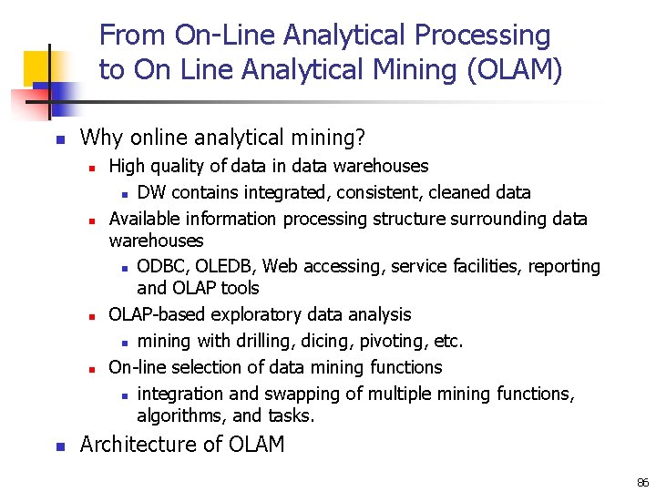
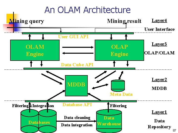
From On-Line Analytical Processing to On Line Analytical Mining (OLAM) n Why online analytical mining? n n n High quality of data in data warehouses n DW contains integrated, consistent, cleaned data Available information processing structure surrounding data warehouses n ODBC, OLEDB, Web accessing, service facilities, reporting and OLAP tools OLAP-based exploratory data analysis n mining with drilling, dicing, pivoting, etc. On-line selection of data mining functions n integration and swapping of multiple mining functions, algorithms, and tasks. Architecture of OLAM 86

An OLAM Architecture Mining query Mining result Layer 4 User Interface User GUI API OLAM Engine OLAP Engine Layer 3 OLAP/OLAM Data Cube API Layer 2 MDDB Meta Data Filtering&Integration Database API Filtering Layer 1 Databases Data cleaning Data integration Warehouse Data Repository 87

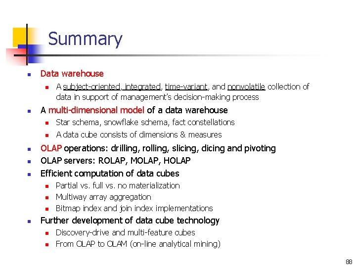
Summary n Data warehouse n n n A multi-dimensional model of a data warehouse n Star schema, snowflake schema, fact constellations n A data cube consists of dimensions & measures OLAP operations: drilling, rolling, slicing, dicing and pivoting OLAP servers: ROLAP, MOLAP, HOLAP Efficient computation of data cubes n n A subject-oriented, integrated, time-variant, and nonvolatile collection of data in support of management’s decision-making process Partial vs. full vs. no materialization Multiway array aggregation Bitmap index and join index implementations Further development of data cube technology n n Discovery-drive and multi-feature cubes From OLAP to OLAM (on-line analytical mining) 88

References (I) n n n n S. Agarwal, R. Agrawal, P. M. Deshpande, A. Gupta, J. F. Naughton, R. Ramakrishnan, and S. Sarawagi. On the computation of multidimensional aggregates. In Proc. 1996 Int. Conf. Very Large Data Bases, 506 -521, Bombay, India, Sept. 1996. D. Agrawal, A. E. Abbadi, A. Singh, and T. Yurek. Efficient view maintenance in data warehouses. In Proc. 1997 ACM-SIGMOD Int. Conf. Management of Data, 417 -427, Tucson, Arizona, May 1997. R. Agrawal, J. Gehrke, D. Gunopulos, and P. Raghavan. Automatic subspace clustering of high dimensional data for data mining applications. In Proc. 1998 ACM-SIGMOD Int. Conf. Management of Data, 94 -105, Seattle, Washington, June 1998. R. Agrawal, A. Gupta, and S. Sarawagi. Modeling multidimensional databases. In Proc. 1997 Int. Conf. Data Engineering, 232 -243, Birmingham, England, April 1997. K. Beyer and R. Ramakrishnan. Bottom-Up Computation of Sparse and Iceberg CUBEs. In Proc. 1999 ACM-SIGMOD Int. Conf. Management of Data (SIGMOD'99), 359 -370, Philadelphia, PA, June 1999. S. Chaudhuri and U. Dayal. An overview of data warehousing and OLAP technology. ACM SIGMOD Record, 26: 65 -74, 1997. OLAP council. MDAPI specification version 2. 0. In http: //www. olapcouncil. org/research/apily. htm, 1998. J. Gray, S. Chaudhuri, A. Bosworth, A. Layman, D. Reichart, M. Venkatrao, F. Pellow, and H. Pirahesh. Data cube: A relational aggregation operator generalizing group-by, cross-tab and subtotals. Data Mining and Knowledge Discovery, 1: 29 -54, 1997. 89

References (II) n n n n V. Harinarayan, A. Rajaraman, and J. D. Ullman. Implementing data cubes efficiently. In Proc. 1996 ACM-SIGMOD Int. Conf. Management of Data, pages 205 -216, Montreal, Canada, June 1996. Microsoft. OLEDB for OLAP programmer's reference version 1. 0. In http: //www. microsoft. com/data/oledb/olap, 1998. K. Ross and D. Srivastava. Fast computation of sparse datacubes. In Proc. 1997 Int. Conf. Very Large Data Bases, 116 -125, Athens, Greece, Aug. 1997. K. A. Ross, D. Srivastava, and D. Chatziantoniou. Complex aggregation at multiple granularities. In Proc. Int. Conf. of Extending Database Technology (EDBT'98), 263 -277, Valencia, Spain, March 1998. S. Sarawagi, R. Agrawal, and N. Megiddo. Discovery-driven exploration of OLAP data cubes. In Proc. Int. Conf. of Extending Database Technology (EDBT'98), pages 168 -182, Valencia, Spain, March 1998. E. Thomsen. OLAP Solutions: Building Multidimensional Information Systems. John Wiley & Sons, 1997. Y. Zhao, P. M. Deshpande, and J. F. Naughton. An array-based algorithm for simultaneous multidimensional aggregates. In Proc. 1997 ACM-SIGMOD Int. Conf. Management of Data, 159 -170, Tucson, Arizona, May 1997. 90