Data Warehousing Data Warehouse and OLAP Technology 1001

Data Warehousing 資料倉儲 Data Warehouse and OLAP Technology 1001 DW 04 MI 4 Tue. 6, 7 (13: 10 -15: 00) B 427 Min-Yuh Day 戴敏育 Assistant Professor 專任助理教授 Dept. of Information Management, Tamkang University 淡江大學 資訊管理學系 http: //mail. im. tku. edu. tw/~myday/ 2011 -09 -27 1

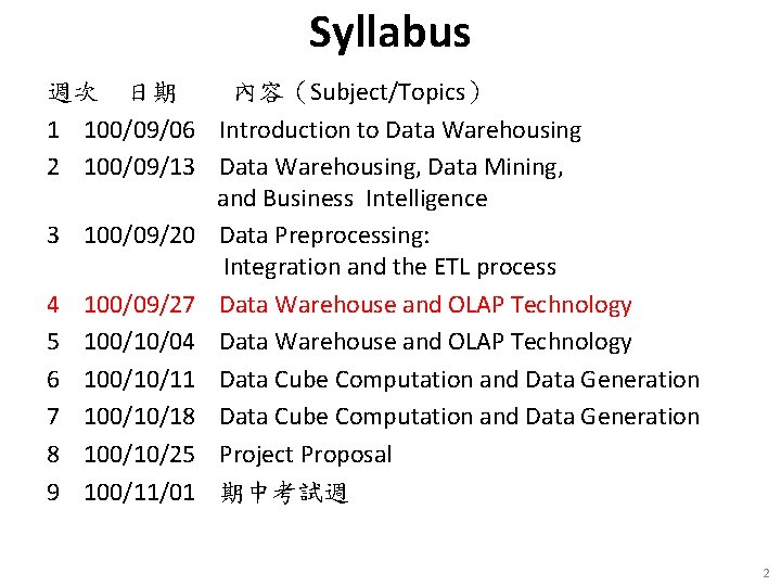
Syllabus 週次 日期 內容（Subject/Topics） 1 100/09/06 Introduction to Data Warehousing 2 100/09/13 Data Warehousing, Data Mining, and Business Intelligence 3 100/09/20 Data Preprocessing: Integration and the ETL process 4 100/09/27 Data Warehouse and OLAP Technology 5 100/10/04 Data Warehouse and OLAP Technology 6 100/10/11 Data Cube Computation and Data Generation 7 100/10/18 Data Cube Computation and Data Generation 8 100/10/25 Project Proposal 9 100/11/01 期中考試週 2

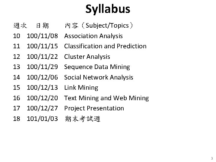
Syllabus 週次 日期 10 100/11/08 11 100/11/15 12 100/11/22 13 100/11/29 14 100/12/06 15 100/12/13 16 100/12/20 17 100/12/27 18 101/01/03 內容（Subject/Topics） Association Analysis Classification and Prediction Cluster Analysis Sequence Data Mining Social Network Analysis Link Mining Text Mining and Web Mining Project Presentation 期末考試週 3

Data Warehouse and OLAP Technology • What is a data warehouse? • A multi-dimensional data model • Data warehouse architecture • Data warehouse implementation • From data warehousing to data mining Source: Han & Kamber (2006) 4

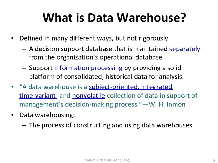
What is Data Warehouse? • Defined in many different ways, but not rigorously. – A decision support database that is maintained separately from the organization’s operational database – Support information processing by providing a solid platform of consolidated, historical data for analysis. • “A data warehouse is a subject-oriented, integrated, time-variant, and nonvolatile collection of data in support of management’s decision-making process. ”—W. H. Inmon • Data warehousing: – The process of constructing and using data warehouses Source: Han & Kamber (2006) 5

Data Warehouse • • Subject-oriented Integrated Time-variant Nonvolatile Source: Han & Kamber (2006) 6

Data Warehouse— Subject-Oriented • Organized around major subjects, such as customer, product, sales • Focusing on the modeling and analysis of data for decision makers, not on daily operations or transaction processing • Provide a simple and concise view around particular subject issues by excluding data that are not useful in the decision support process Source: Han & Kamber (2006) 7

Data Warehouse— Integrated • Constructed by integrating multiple, heterogeneous data sources – relational databases, flat files, on-line transaction records • Data cleaning and data integration techniques are applied. – Ensure consistency in naming conventions, encoding structures, attribute measures, etc. among different data sources • E. g. , Hotel price: currency, tax, breakfast covered, etc. – When data is moved to the warehouse, it is converted. Source: Han & Kamber (2006) 8

Data Warehouse— Time Variant • The time horizon for the data warehouse is significantly longer than that of operational systems – Operational database: current value data – Data warehouse data: provide information from a historical perspective (e. g. , past 5 -10 years) • Every key structure in the data warehouse – Contains an element of time, explicitly or implicitly – But the key of operational data may or may not contain “time element” Source: Han & Kamber (2006) 9

Data Warehouse— Nonvolatile • A physically separate store of data transformed from the operational environment • Operational update of data does not occur in the data warehouse environment – Does not require transaction processing, recovery, and concurrency control mechanisms – Requires only two operations in data accessing: • initial loading of data and access of data Source: Han & Kamber (2006) 10

Data Warehouse vs. Heterogeneous DBMS • Traditional heterogeneous DB integration: A query driven approach – Build wrappers/mediators on top of heterogeneous databases – When a query is posed to a client site, a meta-dictionary is used to translate the query into queries appropriate for individual heterogeneous sites involved, and the results are integrated into a global answer set – Complex information filtering, compete for resources • Data warehouse: update-driven, high performance – Information from heterogeneous sources is integrated in advance and stored in warehouses for direct query and analysis Source: Han & Kamber (2006) 11

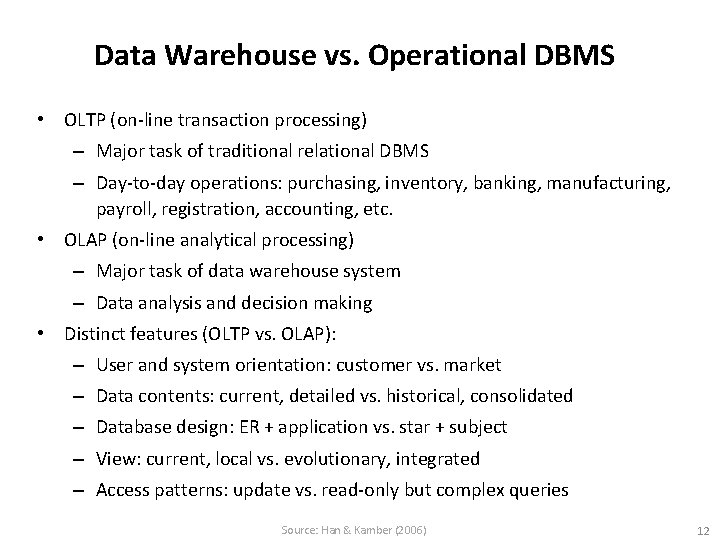
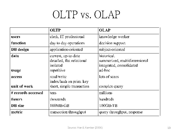
Data Warehouse vs. Operational DBMS • OLTP (on-line transaction processing) – Major task of traditional relational DBMS – Day-to-day operations: purchasing, inventory, banking, manufacturing, payroll, registration, accounting, etc. • OLAP (on-line analytical processing) – Major task of data warehouse system – Data analysis and decision making • Distinct features (OLTP vs. OLAP): – User and system orientation: customer vs. market – Data contents: current, detailed vs. historical, consolidated – Database design: ER + application vs. star + subject – View: current, local vs. evolutionary, integrated – Access patterns: update vs. read-only but complex queries Source: Han & Kamber (2006) 12

OLTP vs. OLAP Source: Han & Kamber (2006) 13

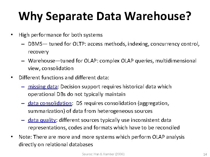
Why Separate Data Warehouse? • High performance for both systems – DBMS— tuned for OLTP: access methods, indexing, concurrency control, recovery – Warehouse—tuned for OLAP: complex OLAP queries, multidimensional view, consolidation • Different functions and different data: – missing data: Decision support requires historical data which operational DBs do not typically maintain – data consolidation: DS requires consolidation (aggregation, summarization) of data from heterogeneous sources – data quality: different sources typically use inconsistent data representations, codes and formats which have to be reconciled • Note: There are more and more systems which perform OLAP analysis directly on relational databases Source: Han & Kamber (2006) 14

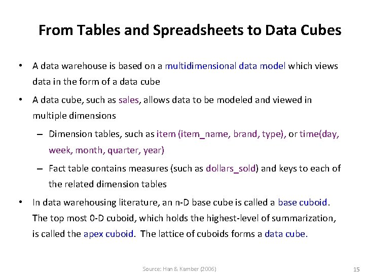
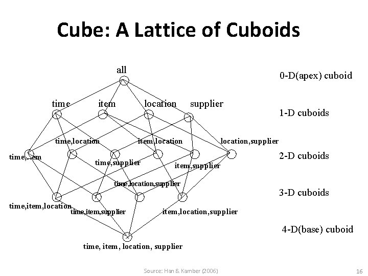
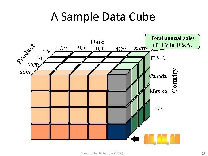
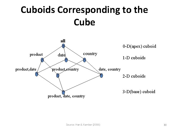
From Tables and Spreadsheets to Data Cubes • A data warehouse is based on a multidimensional data model which views data in the form of a data cube • A data cube, such as sales, allows data to be modeled and viewed in multiple dimensions – Dimension tables, such as item (item_name, brand, type), or time(day, week, month, quarter, year) – Fact table contains measures (such as dollars_sold) and keys to each of the related dimension tables • In data warehousing literature, an n-D base cube is called a base cuboid. The top most 0 -D cuboid, which holds the highest-level of summarization, is called the apex cuboid. The lattice of cuboids forms a data cube. Source: Han & Kamber (2006) 15

Cube: A Lattice of Cuboids all time 0 -D(apex) cuboid item time, location time, item location supplier item, location time, supplier location, supplier item, supplier time, location, supplier time, item, location time, item, supplier 1 -D cuboids 2 -D cuboids 3 -D cuboids item, location, supplier 4 -D(base) cuboid time, item, location, supplier Source: Han & Kamber (2006) 16

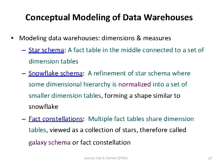
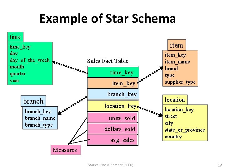
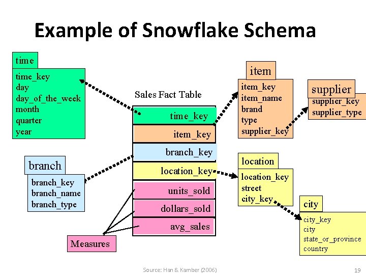
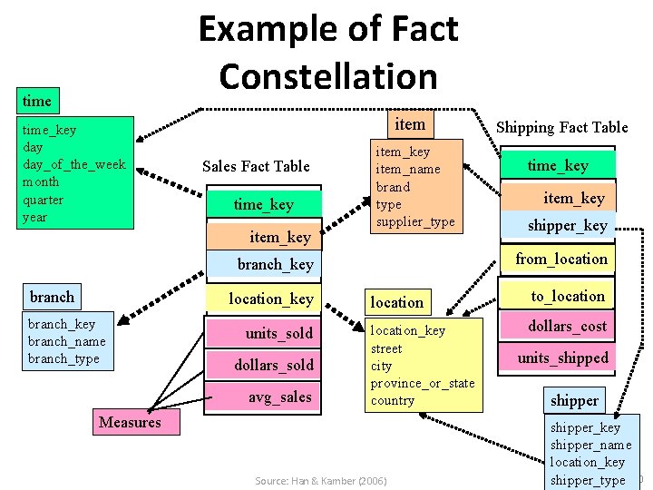
Conceptual Modeling of Data Warehouses • Modeling data warehouses: dimensions & measures – Star schema: A fact table in the middle connected to a set of dimension tables – Snowflake schema: A refinement of star schema where some dimensional hierarchy is normalized into a set of smaller dimension tables, forming a shape similar to snowflake – Fact constellations: Multiple fact tables share dimension tables, viewed as a collection of stars, therefore called galaxy schema or fact constellation Source: Han & Kamber (2006) 17

Example of Star Schema time item time_key day_of_the_week month quarter year Sales Fact Table time_key item_key branch_key branch_name branch_type location_key units_sold dollars_sold avg_sales item_key item_name brand type supplier_type location_key street city state_or_province country Measures Source: Han & Kamber (2006) 18

Example of Snowflake Schema time_key day_of_the_week month quarter year item Sales Fact Table time_key item_key branch location_key branch_name branch_type units_sold dollars_sold avg_sales Measures Source: Han & Kamber (2006) item_key item_name brand type supplier_key supplier_type location_key street city_key city state_or_province country 19

Example of Fact Constellation time_key day_of_the_week month quarter year item Sales Fact Table time_key item_key item_name brand type supplier_type location_key branch_name branch_type units_sold dollars_sold avg_sales time_key item_key shipper_key from_location branch_key branch Shipping Fact Table location to_location_key street city province_or_state country dollars_cost Measures Source: Han & Kamber (2006) units_shipped shipper_key shipper_name location_key shipper_type 20

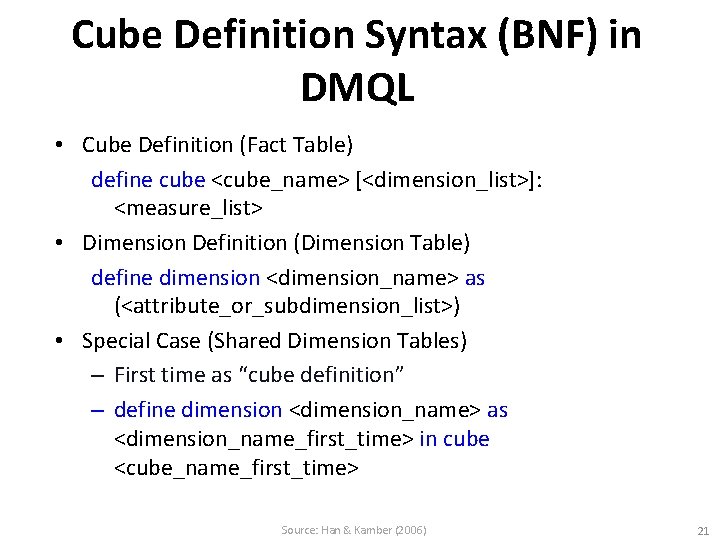
Cube Definition Syntax (BNF) in DMQL • Cube Definition (Fact Table) define cube <cube_name> [<dimension_list>]: <measure_list> • Dimension Definition (Dimension Table) define dimension <dimension_name> as (<attribute_or_subdimension_list>) • Special Case (Shared Dimension Tables) – First time as “cube definition” – define dimension <dimension_name> as <dimension_name_first_time> in cube <cube_name_first_time> Source: Han & Kamber (2006) 21

Defining Star Schema in DMQL define cube sales_star [time, item, branch, location]: dollars_sold = sum(sales_in_dollars), avg_sales = avg(sales_in_dollars), units_sold = count(*) define dimension time as (time_key, day_of_week, month, quarter, year) define dimension item as (item_key, item_name, brand, type, supplier_type) define dimension branch as (branch_key, branch_name, branch_type) define dimension location as (location_key, street, city, province_or_state, country) Source: Han & Kamber (2006) 22

Defining Snowflake Schema in DMQL define cube sales_snowflake [time, item, branch, location]: dollars_sold = sum(sales_in_dollars), avg_sales = avg(sales_in_dollars), units_sold = count(*) define dimension time as (time_key, day_of_week, month, quarter, year) define dimension item as (item_key, item_name, brand, type, supplier(supplier_key, supplier_type)) define dimension branch as (branch_key, branch_name, branch_type) define dimension location as (location_key, street, city(city_key, province_or_state, country)) Source: Han & Kamber (2006) 23

Defining Fact Constellation in DMQL define cube sales [time, item, branch, location]: dollars_sold = sum(sales_in_dollars), avg_sales = avg(sales_in_dollars), units_sold = count(*) define dimension time as (time_key, day_of_week, month, quarter, year) define dimension item as (item_key, item_name, brand, type, supplier_type) define dimension branch as (branch_key, branch_name, branch_type) define dimension location as (location_key, street, city, province_or_state, country) define cube shipping [time, item, shipper, from_location, to_location]: dollar_cost = sum(cost_in_dollars), unit_shipped = count(*) define dimension time as time in cube sales define dimension item as item in cube sales define dimension shipper as (shipper_key, shipper_name, location as location in cube sales, shipper_type) define dimension from_location as location in cube sales define dimension to_location as location in cube sales Source: Han & Kamber (2006) 24

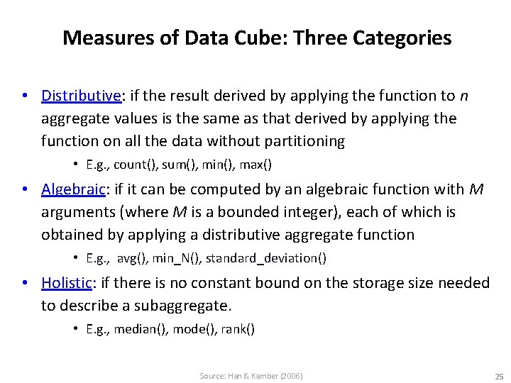
Measures of Data Cube: Three Categories • Distributive: if the result derived by applying the function to n aggregate values is the same as that derived by applying the function on all the data without partitioning • E. g. , count(), sum(), min(), max() • Algebraic: if it can be computed by an algebraic function with M arguments (where M is a bounded integer), each of which is obtained by applying a distributive aggregate function • E. g. , avg(), min_N(), standard_deviation() • Holistic: if there is no constant bound on the storage size needed to describe a subaggregate. • E. g. , median(), mode(), rank() Source: Han & Kamber (2006) 25

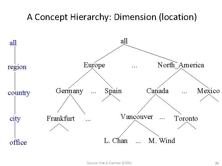
A Concept Hierarchy: Dimension (location) all Europe region country city office Germany Frankfurt . . Spain North_America Canada Vancouver. . . L. Chan Source: Han & Kamber (2006) . . . Mexico Toronto M. Wind 26

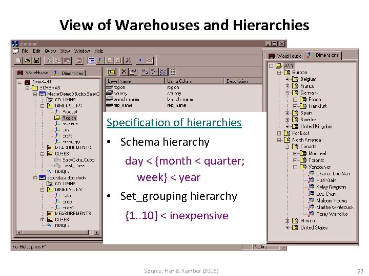
View of Warehouses and Hierarchies Specification of hierarchies • Schema hierarchy day < {month < quarter; week} < year • Set_grouping hierarchy {1. . 10} < inexpensive Source: Han & Kamber (2006) 27

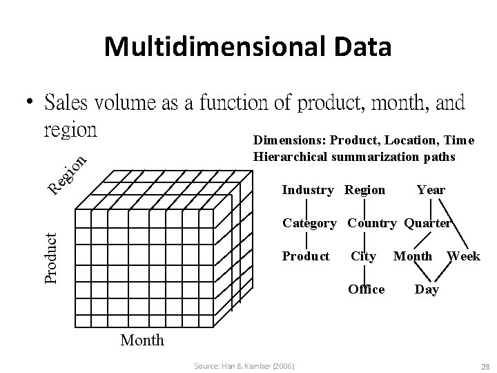
Multidimensional Data • Sales volume as a function of product, month, and region Dimensions: Product, Location, Time gi on Hierarchical summarization paths Re Industry Region Year Product Category Country Quarter Product City Month Week Office Day Month Source: Han & Kamber (2006) 28

2 Qtr 3 Qtr 4 Qtr od TV PC VCR sum 1 Qtr Date sum Total annual sales of TV in U. S. A. Pr U. S. A Canada Mexico Country uc t A Sample Data Cube sum Source: Han & Kamber (2006) 29

Cuboids Corresponding to the Cube all 0 -D(apex) cuboid product, date country date product, country 1 -D cuboids date, country 2 -D cuboids product, date, country Source: Han & Kamber (2006) 3 -D(base) cuboid 30

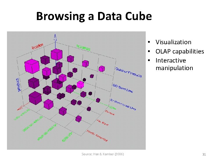
Browsing a Data Cube • Visualization • OLAP capabilities • Interactive manipulation Source: Han & Kamber (2006) 31

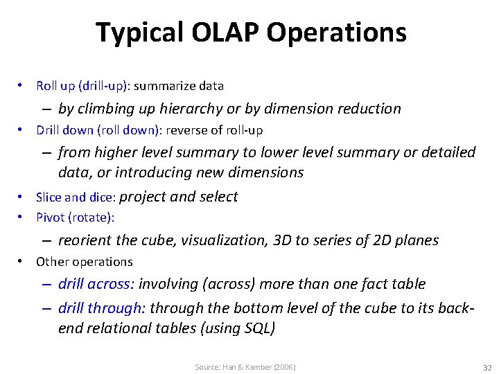
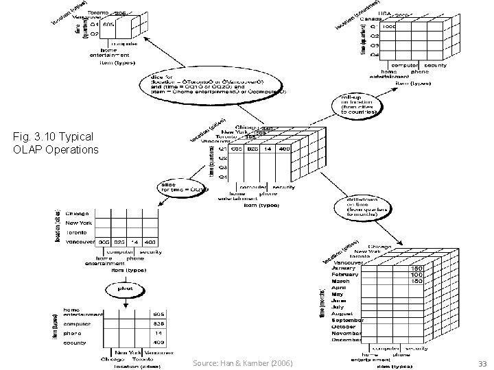
Typical OLAP Operations • Roll up (drill-up): summarize data – by climbing up hierarchy or by dimension reduction • Drill down (roll down): reverse of roll-up – from higher level summary to lower level summary or detailed data, or introducing new dimensions • Slice and dice: project and select • Pivot (rotate): – reorient the cube, visualization, 3 D to series of 2 D planes • Other operations – drill across: involving (across) more than one fact table – drill through: through the bottom level of the cube to its backend relational tables (using SQL) Source: Han & Kamber (2006) 32

Fig. 3. 10 Typical OLAP Operations Source: Han & Kamber (2006) 33

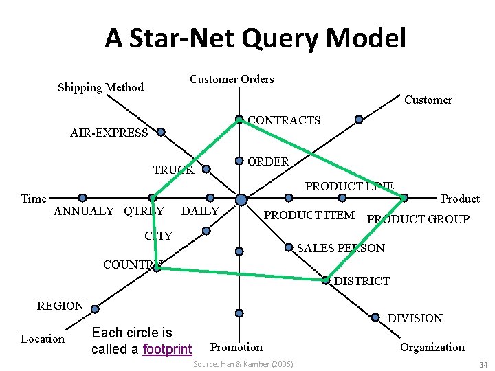
A Star-Net Query Model Customer Orders Shipping Method Customer CONTRACTS AIR-EXPRESS ORDER TRUCK Time PRODUCT LINE ANNUALY QTRLY DAILY Product PRODUCT ITEM PRODUCT GROUP CITY SALES PERSON COUNTRY DISTRICT REGION Location Each circle is called a footprint DIVISION Promotion Source: Han & Kamber (2006) Organization 34

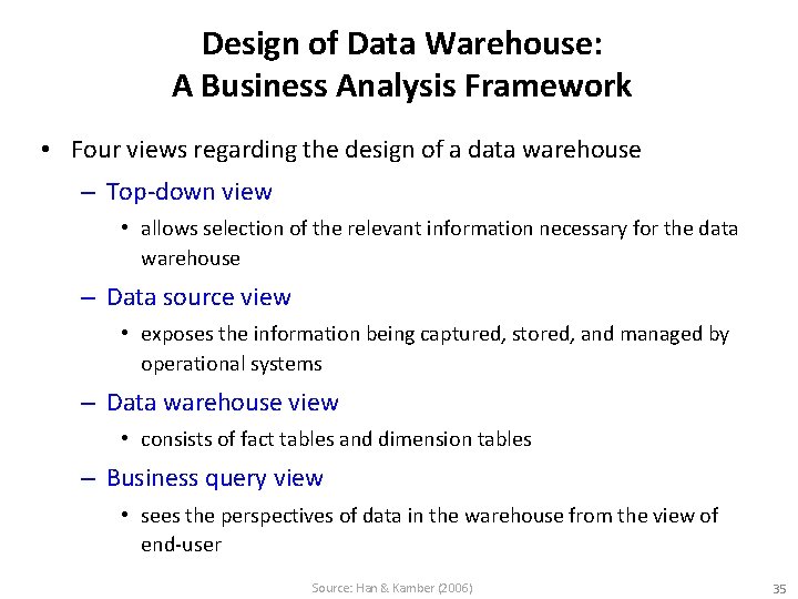
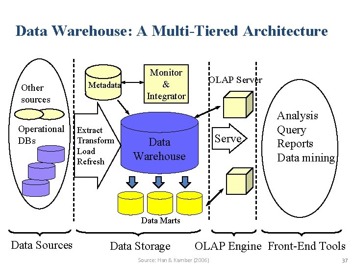
Design of Data Warehouse: A Business Analysis Framework • Four views regarding the design of a data warehouse – Top-down view • allows selection of the relevant information necessary for the data warehouse – Data source view • exposes the information being captured, stored, and managed by operational systems – Data warehouse view • consists of fact tables and dimension tables – Business query view • sees the perspectives of data in the warehouse from the view of end-user Source: Han & Kamber (2006) 35

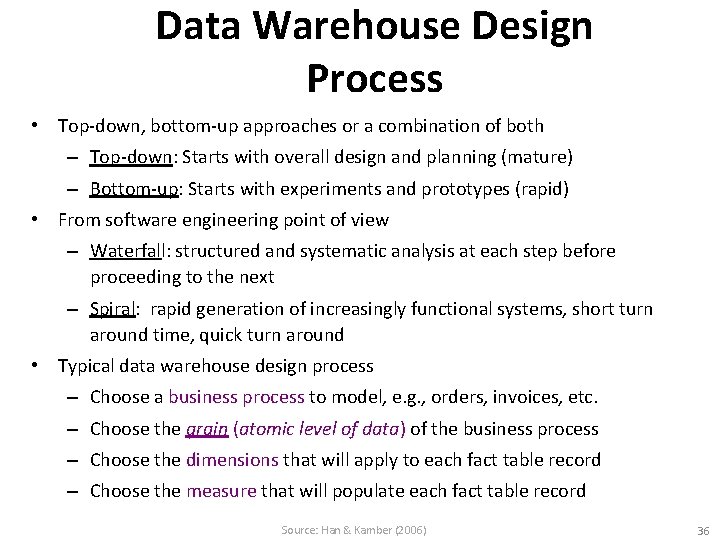
Data Warehouse Design Process • Top-down, bottom-up approaches or a combination of both – Top-down: Starts with overall design and planning (mature) – Bottom-up: Starts with experiments and prototypes (rapid) • From software engineering point of view – Waterfall: structured and systematic analysis at each step before proceeding to the next – Spiral: rapid generation of increasingly functional systems, short turn around time, quick turn around • Typical data warehouse design process – Choose a business process to model, e. g. , orders, invoices, etc. – Choose the grain (atomic level of data) of the business process – Choose the dimensions that will apply to each fact table record – Choose the measure that will populate each fact table record Source: Han & Kamber (2006) 36

Data Warehouse: A Multi-Tiered Architecture Other sources Operational DBs Metadata Extract Transform Load Refresh Monitor & Integrator OLAP Server Serve Data Warehouse Analysis Query Reports Data mining Data Marts Data Sources Data Storage OLAP Engine Front-End Tools Source: Han & Kamber (2006) 37

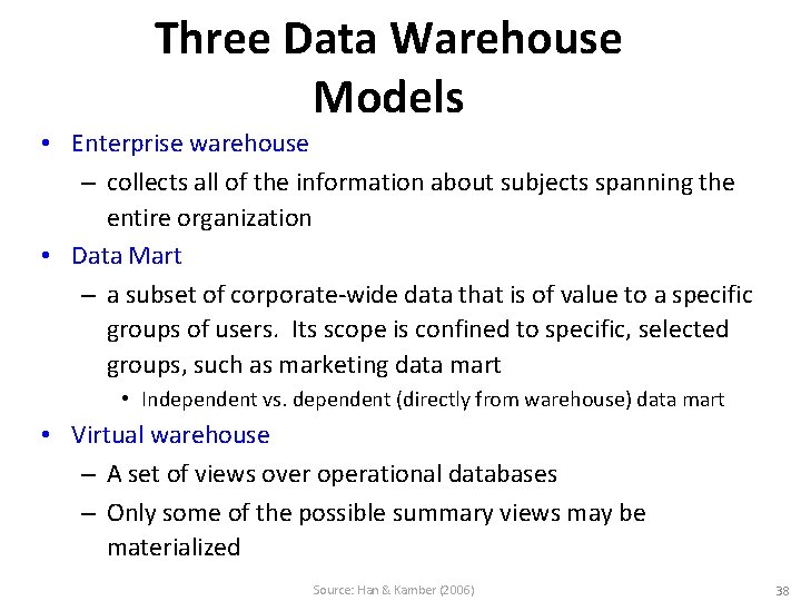
Three Data Warehouse Models • Enterprise warehouse – collects all of the information about subjects spanning the entire organization • Data Mart – a subset of corporate-wide data that is of value to a specific groups of users. Its scope is confined to specific, selected groups, such as marketing data mart • Independent vs. dependent (directly from warehouse) data mart • Virtual warehouse – A set of views over operational databases – Only some of the possible summary views may be materialized Source: Han & Kamber (2006) 38

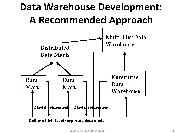
Data Warehouse Development: A Recommended Approach Multi-Tier Data Warehouse Distributed Data Marts Data Mart Model refinement Enterprise Data Warehouse Model refinement Define a high-level corporate data model Source: Han & Kamber (2006) 39

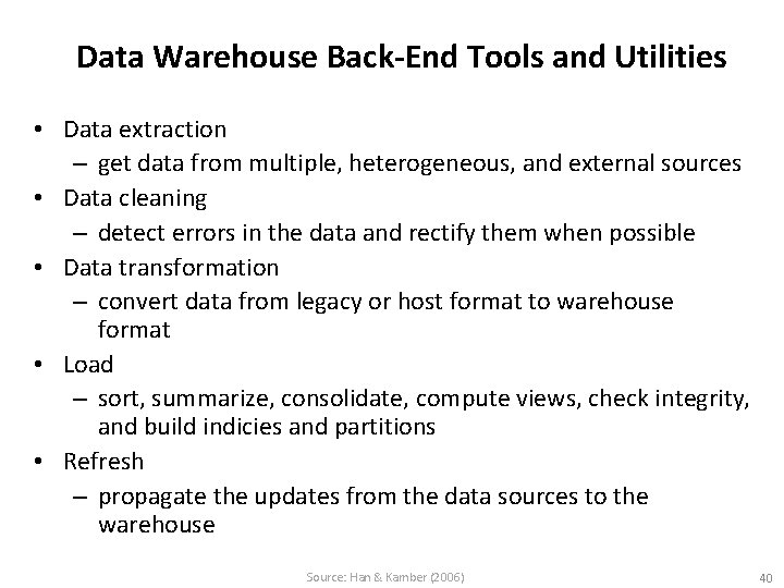
Data Warehouse Back-End Tools and Utilities • Data extraction – get data from multiple, heterogeneous, and external sources • Data cleaning – detect errors in the data and rectify them when possible • Data transformation – convert data from legacy or host format to warehouse format • Load – sort, summarize, consolidate, compute views, check integrity, and build indicies and partitions • Refresh – propagate the updates from the data sources to the warehouse Source: Han & Kamber (2006) 40

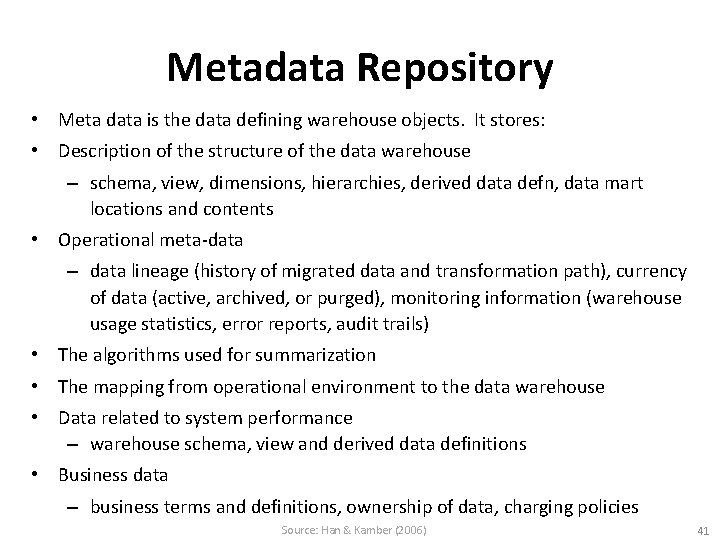
Metadata Repository • Meta data is the data defining warehouse objects. It stores: • Description of the structure of the data warehouse – schema, view, dimensions, hierarchies, derived data defn, data mart locations and contents • Operational meta-data – data lineage (history of migrated data and transformation path), currency of data (active, archived, or purged), monitoring information (warehouse usage statistics, error reports, audit trails) • The algorithms used for summarization • The mapping from operational environment to the data warehouse • Data related to system performance – warehouse schema, view and derived data definitions • Business data – business terms and definitions, ownership of data, charging policies Source: Han & Kamber (2006) 41

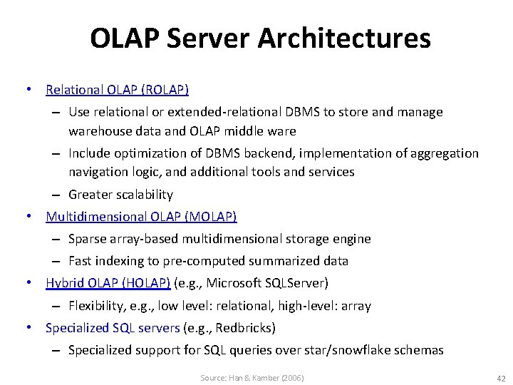
OLAP Server Architectures • Relational OLAP (ROLAP) – Use relational or extended-relational DBMS to store and manage warehouse data and OLAP middle ware – Include optimization of DBMS backend, implementation of aggregation navigation logic, and additional tools and services – Greater scalability • Multidimensional OLAP (MOLAP) – Sparse array-based multidimensional storage engine – Fast indexing to pre-computed summarized data • Hybrid OLAP (HOLAP) (e. g. , Microsoft SQLServer) – Flexibility, e. g. , low level: relational, high-level: array • Specialized SQL servers (e. g. , Redbricks) – Specialized support for SQL queries over star/snowflake schemas Source: Han & Kamber (2006) 42

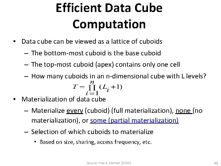
Efficient Data Cube Computation • Data cube can be viewed as a lattice of cuboids – The bottom-most cuboid is the base cuboid – The top-most cuboid (apex) contains only one cell – How many cuboids in an n-dimensional cube with L levels? • Materialization of data cube – Materialize every (cuboid) (full materialization), none (no materialization), or some (partial materialization) – Selection of which cuboids to materialize • Based on size, sharing, access frequency, etc. Source: Han & Kamber (2006) 43

Cube Operation • Cube definition and computation in DMQL define cube sales[item, city, year]: sum(sales_in_dollars) compute cube sales • Transform it into a SQL-like language (with a new operator cube by, introduced by Gray et al. ’ 96) () SELECT item, city, year, SUM (amount) (city) FROM SALES (item) (year) CUBE BY item, city, year • Need compute the following Group-Bys (city, item) (city, year) (item, year) (date, product, customer), (date, product), (date, customer), (product, customer), (date), (product), (customer) (city, item, year) () Source: Han & Kamber (2006) 44

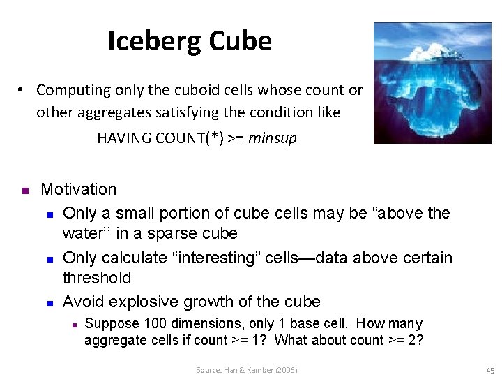
Iceberg Cube • Computing only the cuboid cells whose count or other aggregates satisfying the condition like HAVING COUNT(*) >= minsup n Motivation n Only a small portion of cube cells may be “above the water’’ in a sparse cube n Only calculate “interesting” cells—data above certain threshold n Avoid explosive growth of the cube n Suppose 100 dimensions, only 1 base cell. How many aggregate cells if count >= 1? What about count >= 2? Source: Han & Kamber (2006) 45

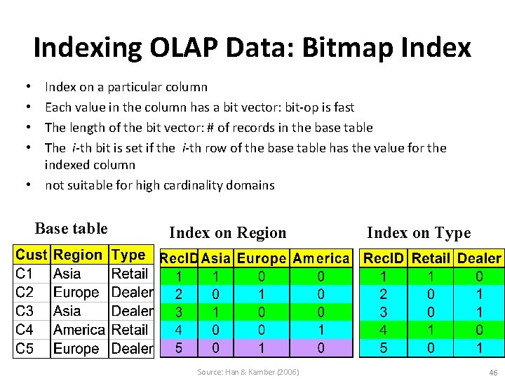
Indexing OLAP Data: Bitmap Index on a particular column Each value in the column has a bit vector: bit-op is fast The length of the bit vector: # of records in the base table The i-th bit is set if the i-th row of the base table has the value for the indexed column • not suitable for high cardinality domains • • Base table Index on Region Source: Han & Kamber (2006) Index on Type 46

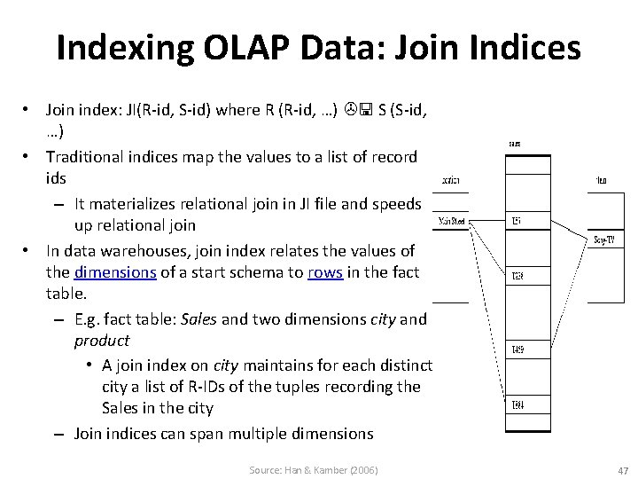
Indexing OLAP Data: Join Indices • Join index: JI(R-id, S-id) where R (R-id, …) S (S-id, …) • Traditional indices map the values to a list of record ids – It materializes relational join in JI file and speeds up relational join • In data warehouses, join index relates the values of the dimensions of a start schema to rows in the fact table. – E. g. fact table: Sales and two dimensions city and product • A join index on city maintains for each distinct city a list of R-IDs of the tuples recording the Sales in the city – Join indices can span multiple dimensions Source: Han & Kamber (2006) 47

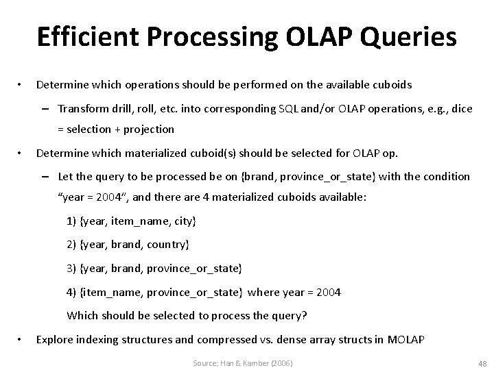
Efficient Processing OLAP Queries • Determine which operations should be performed on the available cuboids – Transform drill, roll, etc. into corresponding SQL and/or OLAP operations, e. g. , dice = selection + projection • Determine which materialized cuboid(s) should be selected for OLAP op. – Let the query to be processed be on {brand, province_or_state} with the condition “year = 2004”, and there are 4 materialized cuboids available: 1) {year, item_name, city} 2) {year, brand, country} 3) {year, brand, province_or_state} 4) {item_name, province_or_state} where year = 2004 Which should be selected to process the query? • Explore indexing structures and compressed vs. dense array structs in MOLAP Source: Han & Kamber (2006) 48

From data warehousing to data mining Source: Han & Kamber (2006) 49

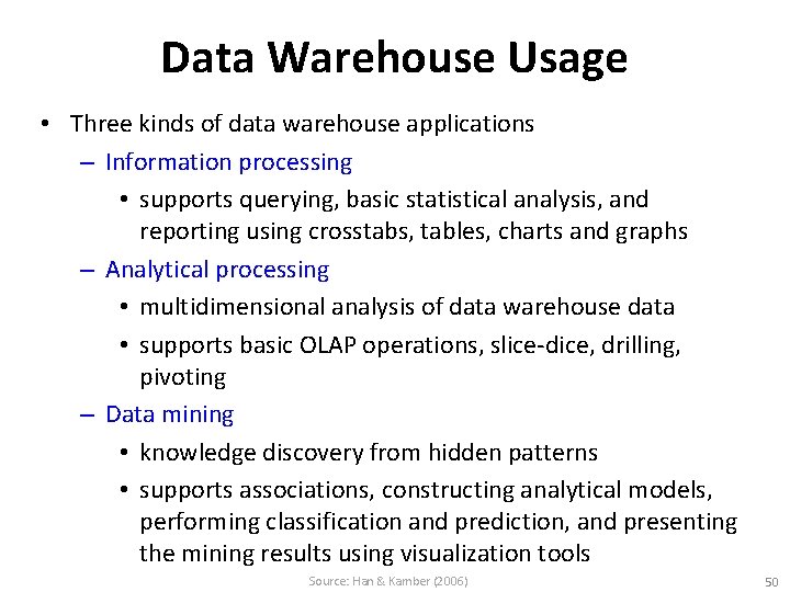
Data Warehouse Usage • Three kinds of data warehouse applications – Information processing • supports querying, basic statistical analysis, and reporting using crosstabs, tables, charts and graphs – Analytical processing • multidimensional analysis of data warehouse data • supports basic OLAP operations, slice-dice, drilling, pivoting – Data mining • knowledge discovery from hidden patterns • supports associations, constructing analytical models, performing classification and prediction, and presenting the mining results using visualization tools Source: Han & Kamber (2006) 50

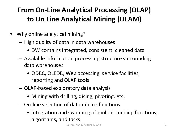
From On-Line Analytical Processing (OLAP) to On Line Analytical Mining (OLAM) • Why online analytical mining? – High quality of data in data warehouses • DW contains integrated, consistent, cleaned data – Available information processing structure surrounding data warehouses • ODBC, OLEDB, Web accessing, service facilities, reporting and OLAP tools – OLAP-based exploratory data analysis • Mining with drilling, dicing, pivoting, etc. – On-line selection of data mining functions • Integration and swapping of multiple mining functions, algorithms, and tasks Source: Han & Kamber (2006) 51

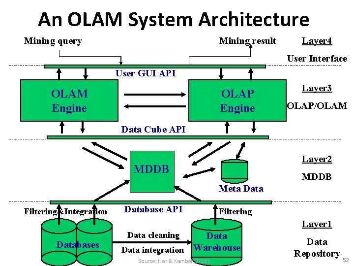
An OLAM System Architecture Mining query Mining result Layer 4 User Interface User GUI API OLAM Engine OLAP Engine Layer 3 OLAP/OLAM Data Cube API Layer 2 MDDB Meta Data Filtering&Integration Database API Filtering Layer 1 Databases Data cleaning Data integration Warehouse Source: Han & Kamber (2006) Data Repository 52

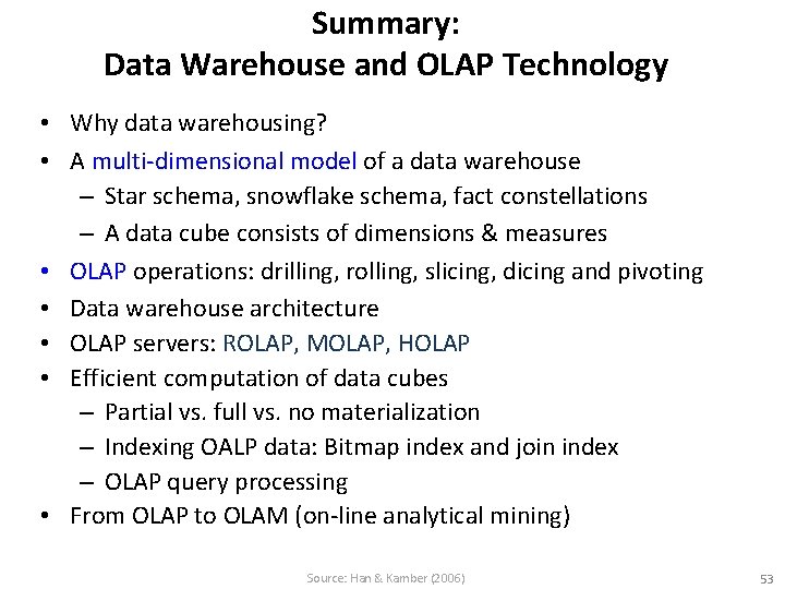
Summary: Data Warehouse and OLAP Technology • Why data warehousing? • A multi-dimensional model of a data warehouse – Star schema, snowflake schema, fact constellations – A data cube consists of dimensions & measures • OLAP operations: drilling, rolling, slicing, dicing and pivoting • Data warehouse architecture • OLAP servers: ROLAP, MOLAP, HOLAP • Efficient computation of data cubes – Partial vs. full vs. no materialization – Indexing OALP data: Bitmap index and join index – OLAP query processing • From OLAP to OLAM (on-line analytical mining) Source: Han & Kamber (2006) 53

References • Jiawei Han and Micheline Kamber, Data Mining: Concepts and Techniques, Second Edition, 2006, Elsevier • Efraim Turban, Ramesh Sharda, Dursun Delen, Decision Support and Business Intelligence Systems, Ninth Edition, 2011, Pearson. 54