Data Mining Lecture 5 Course Syllabus Case Study

Data Mining Lecture 5

Course Syllabus • Case Study 1: Working and experiencing on the properties of The Retail Banking Data Mart (Week 4 – Assignment 1) • Data Analysis Techniques (Week 5) – – Statistical Background Trends/ Outliers/Normalizations Principal Component Analysis Discretization Techniques • Case Study 2: Working and experiencing on the properties of discretization infrastructure of The Retail Banking Data Mart (Week 5 –Assignment 2) • Lecture Talk: Searching/Matching Engine

The importance of Statistics • Why we need to use descriptive summaries? – Motivation • – Data dispersion characteristics • – – To better understand the data: central tendency, variation and spread median, max, min, quantiles, outliers, variance, etc. Numerical dimensions correspond to sorted intervals • Data dispersion: analyzed with multiple granularities of precision • Boxplot or quantile analysis on sorted intervals Dispersion analysis on computed measures • Folding measures into numerical dimensions • Boxplot or quantile analysis on the transformed cube

Remember Stats Facts • Min: – What is the big oh value for finding min of n-sized list ? • Max: – What is the min number of comparisons needed to find the max of n -sized list? • Range: – Max-Min – What about simultaneous finding of min-max? • Value Types: – – Cardinal value -> how many, counting numbers Nominal value -> names and identifies something Ordinal value -> order of things, rank, position Continuous value -> real number
 (sample vs. population): – Weighted arithmetic mean:")
Remember Stats Facts • Mean (algebraic measure) (sample vs. population): – Weighted arithmetic mean: – Trimmed mean: chopping extreme values • Median: A holistic measure – Middle value if odd number of values, or average of the middle two values otherwise – Estimated by interpolation (for grouped data): • Mode – Value that occurs most frequently in the data – Unimodal, bimodal, trimodal – Empirical formula:
![Transformation • Min-max normalization: to [new_min. A, new_max. A] – Ex. Let income range](http://slidetodoc.com/presentation_image_h/dba4d4d98f4ceeb751b92e02f82cf393/image-6.jpg "Transformation • Min-max normalization: to [new_min. A, new_max. A] – Ex. Let income range")
Transformation • Min-max normalization: to [new_min. A, new_max. A] – Ex. Let income range $12, 000 to $98, 000 normalized to [0. 0, 1. 0]. Then $73, 600 is mapped to • Z-score normalization (μ: mean, σ: standard deviation): • Ex. Let μ = 54, 000, σ = 16, 000. Then • Normalization by decimal scaling Where j is the smallest integer such that Max(|ν’|) < 1

The importance of Mean and Median: figuring out the shape of the distribution symmetric mean > median > mode positively skewed mean < median < mode negatively skewed

Measuring dispersion of data Quantiles: Quantiles are points taken at regular intervals from the cumulative distribution function (CDF) of a random variable. Dividing ordered data into q essentially equal-sized data subsets is the motivation for q-quantiles; the quantiles are the data values marking the boundaries between consecutive subsets The 1000 -quantiles are called permillages --> Pr The 100 -quantiles are called percentiles --> P The 20 -quantiles are called vigiciles --> V The 12 -quantiles are called duo-deciles --> Dd The 10 -quantiles are called deciles --> D The 9 -quantiles are called noniles (common in educational testing)--> NO The 5 -quantiles are called quintiles --> QU The 4 -quantiles are called quartiles --> Q The 3 -quantiles are called tertiles or terciles --> T

Measuring dispersion of data k th standardized moment • The first standardized moment is zero, because the first moment about the mean is zero • The second standardized moment is one, because the second moment about the mean is equal to the variance (the square of the standard deviation) • The third standardized moment is the skewness (seen before) • The fourth standardized moment is the kurtosis (estimate peak structure)
,")
Measuring dispersion of data Quartiles, outliers and boxplots Quartiles: Q 1 (25 th percentile), Q 3 (75 th percentile) Inter-quartile range: IQR = Q 3 – Q 1 Five number summary: min, Q 1, MEDIAN, Q 3, max Boxplot: ends of the box are the quartiles, median is marked, whiskers, and plot outlier individually Outlier: usually, a value higher/lower than 1. 5 x IQR Variance and standard deviation (sample: s, population: σ) Variance: (algebraic, scalable computation) Standard deviation s (or σ) is the square root of variance s 2 (or σ2)

Measuring dispersion of data What is the difference between sample variance, standart variance, What is the use of N-1 in s formula ? Does it make sense ? Bessel’s correction or degrees of freedom the sample error of a hypothesis with respect to some sample S of instances drawn from X is the fraction of S that it misclassifies the true error of a hypothesis is the probability that it will misclassify a single randomly drawn instance from the distribution D Estimation bias (difference between true error and sample error)

Measuring dispersion of data

Measuring dispersion of data

Measuring dispersion of data Chebiyshev Inequality Let X be a random variable with expected value μ and finite variance σ2. Then for any real number k > 0, Only the cases k > 1 provide useful information. This can be equivalently stated as At least 50% of the values are within √ 2 standard deviations from the mean. At least 75% of the values are within 2 standard deviations from the mean. At least 89% of the values are within 3 standard deviations from the mean. At least 94% of the values are within 4 standard deviations from the mean. At least 96% of the values are within 5 standard deviations from the mean. At least 97% of the values are within 6 standard deviations from the mean. At least 98% of the values are within 7 standard deviations from the mean.
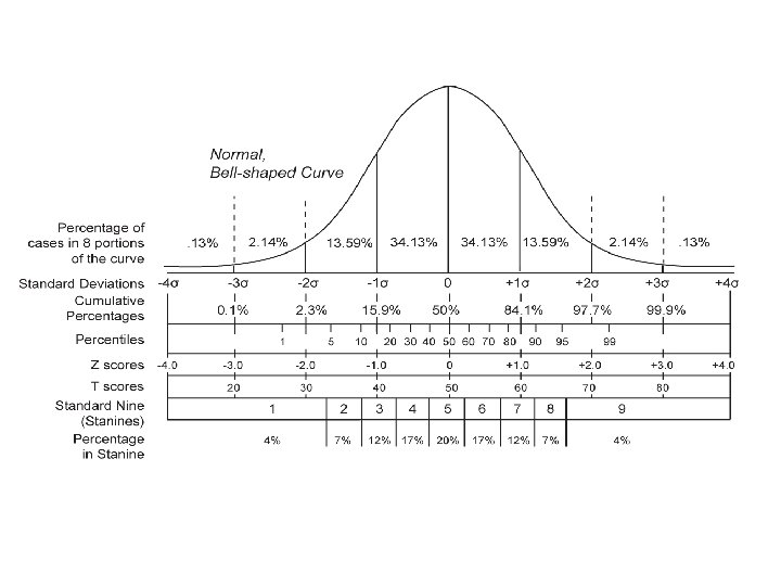
 curve – From μ–σ to μ+σ:")
Measuring dispersion of data • The normal (distribution) curve – From μ–σ to μ+σ: contains about 68% of the measurements (μ: mean, σ: standard deviation) – From μ– 2σ to μ+2σ: contains about 95% of it – From μ– 3σ to μ+3σ: contains about 99. 7% of it

Boxplot Analysis • Five-number summary of a distribution: – Minimum, Q 1, M, Q 3, Maximum • Boxplot – Data is represented with a box – The ends of the box are at the first and third quartiles, i. e. , the height of the box is IRQ – The median is marked by a line within the box – Whiskers: two lines outside the box extend to Minimum and Maximum

Histogram Analysis • Graph displays of basic statistical class descriptions – Frequency histograms • A univariate graphical method • Consists of a set of rectangles that reflect the counts or frequencies of the classes present in the given data

Quantile Plot • Displays all of the data (allowing the user to assess both the overall behavior and unusual occurrences) • Plots quantile information – For a data xi data sorted in increasing order, fi indicates that approximately 100 fi% of the data are below or equal to the value xi

Scatter plot • Provides a first look at bivariate data to see clusters of points, outliers, etc • Each pair of values is treated as a pair of coordinates and plotted as points in the plane

Loess Curve • Adds a smooth curve to a scatter plot in order to provide better perception of the pattern of dependence • Loess curve is fitted by setting two parameters: a smoothing parameter, and the degree of the polynomials that are fitted by the regression

Covarience The covariance between two real-valued random variables X and Y, with expected values and is defined as Understanding the correlationship
 • Correlation coefficient (also called Pearson’s product moment coefficient) –")
Correlation Analysis (Numerical Data) • Correlation coefficient (also called Pearson’s product moment coefficient) – where n is the number of tuples, and are the respective means of A and B, σA and σB are the respective standard deviation of A and B, and Σ(AB) is the sum of the AB cross-product. • If r. A, B > 0, A and B are positively correlated (A’s values increase as B’s). The higher, the stronger correlation. • r. A, B = 0: independent; r. A, B < 0: negatively correlated
 • Χ 2 (chi-square) test (we will return back again)")
Correlation Analysis (Categorical Data) • Χ 2 (chi-square) test (we will return back again) • The larger the Χ 2 value, the more likely the variables are related • The cells that contribute the most to the Χ 2 value are those whose actual count is very different from the expected count
 • • Given N data vectors from n-dimensions,")
Dimensionality Reduction: Principal Component Analysis (PCA) • • Given N data vectors from n-dimensions, find k ≤ n orthogonal vectors (principal components) that can be best used to represent data Steps – Normalize input data: Each attribute falls within the same range – Compute k orthonormal (unit) vectors, i. e. , principal components – Each input data (vector) is a linear combination of the k principal component vectors – The principal components are sorted in order of decreasing “significance” or strength – Since the components are sorted, the size of the data can be reduced by eliminating the weak components, i. e. , those with low variance. (i. e. , using the strongest principal components, it is possible to reconstruct a good approximation of the original data Works for numeric data only Used when the number of dimensions is large

Principal Component Analysis X 2 Y 1 Y 2 X 1
: Histograms • Divide data into buckets and store average (sum)")
Data Reduction Method (2): Histograms • Divide data into buckets and store average (sum) for each bucket • Partitioning rules: – Equal-width: equal bucket range – Equal-frequency (or equal-depth) • Partition data set into clusters based on similarity, and store cluster representation (e. g. , centroid and diameter) only

Sampling: Cluster or Stratified Sampling Raw Data Cluster/Stratified Sample

Discretization • Discretization: – Divide the range of a continuous attribute into intervals – Some classification algorithms only accept categorical attributes. – Reduce data size by discretization – Prepare for further analysis

Discretization and Concept Hierarchy • Discretization – Reduce the number of values for a given continuous attribute by dividing the range of the attribute into intervals – Interval labels can then be used to replace actual data values – Supervised vs. unsupervised – Split (top-down) vs. merge (bottom-up) – Discretization can be performed recursively on an attribute • Concept hierarchy formation – Recursively reduce the data by collecting and replacing low level concepts (such as numeric values for age) by higher level concepts (such as young, middle-aged, or senior)
 –")
Week 5 -End • assignment 1 (please share your ideas with your group) – choose freely a dataset my advice: http: //www. inf. ed. ac. uk/teaching/courses/dme/html/dat asets 0405. html - evaluate every attribute get descriptive statistics find mean, median, max, range, min, histogram, quartile, percentile, determine missing value strategy, erraneous value strategy, inconsistent value strategy - you can freely use any Statistics Tool. But my advice use open source Weka http: //www. cs. waikato. ac. nz/ml/weka/

Week 5 -End • read – Course Text Book Chapter 2 – Supplemantary Book “Machine Learning”- Tom Mitchell Chapter 5
- Slides: 32