Data Integration Concluded Physical Data Storage Zachary G

Data Integration, Concluded Physical Data Storage Zachary G. Ives University of Pennsylvania CIS 550 – Database & Information Systems

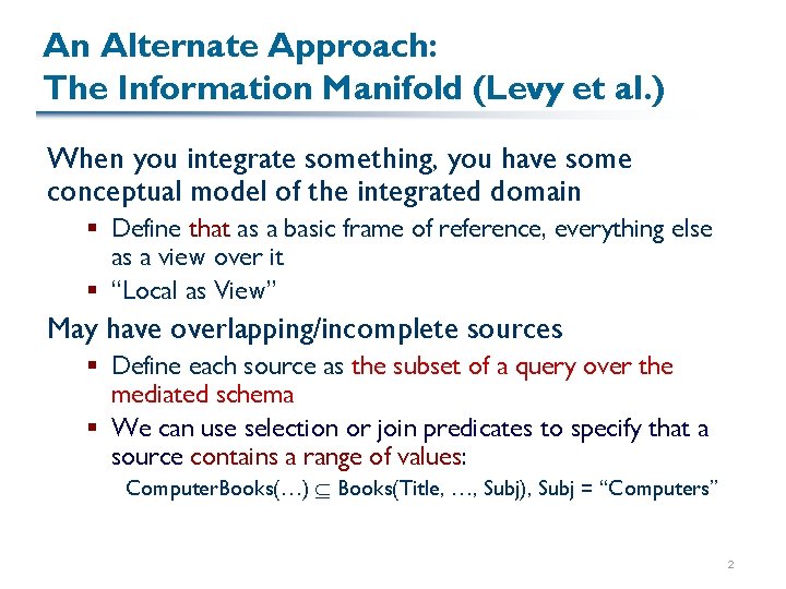
An Alternate Approach: The Information Manifold (Levy et al. ) When you integrate something, you have some conceptual model of the integrated domain § Define that as a basic frame of reference, everything else as a view over it § “Local as View” May have overlapping/incomplete sources § Define each source as the subset of a query over the mediated schema § We can use selection or join predicates to specify that a source contains a range of values: Computer. Books(…) Books(Title, …, Subj), Subj = “Computers” 2

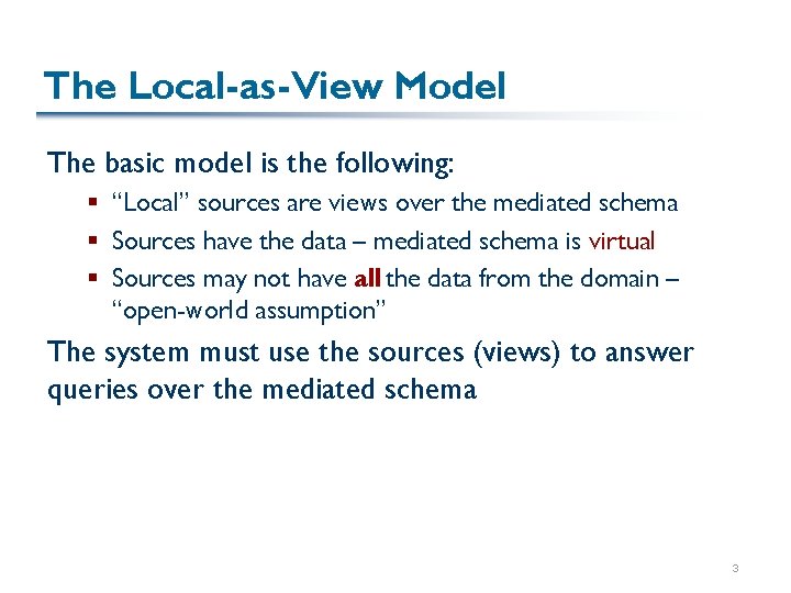
The Local-as-View Model The basic model is the following: § “Local” sources are views over the mediated schema § Sources have the data – mediated schema is virtual § Sources may not have all the data from the domain – “open-world assumption” The system must use the sources (views) to answer queries over the mediated schema 3

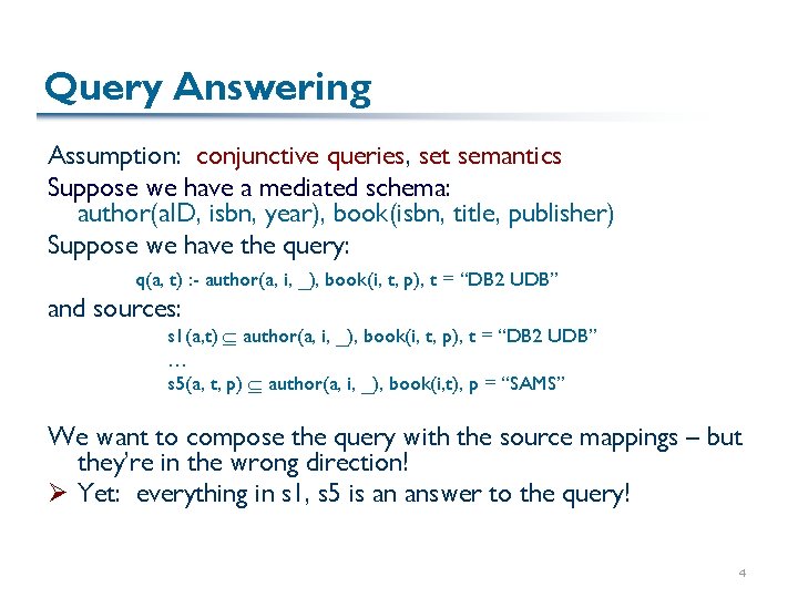
Query Answering Assumption: conjunctive queries, set semantics Suppose we have a mediated schema: author(a. ID, isbn, year), book(isbn, title, publisher) Suppose we have the query: q(a, t) : - author(a, i, _), book(i, t, p), t = “DB 2 UDB” and sources: s 1(a, t) author(a, i, _), book(i, t, p), t = “DB 2 UDB” … s 5(a, t, p) author(a, i, _), book(i, t), p = “SAMS” We want to compose the query with the source mappings – but they’re in the wrong direction! Ø Yet: everything in s 1, s 5 is an answer to the query! 4

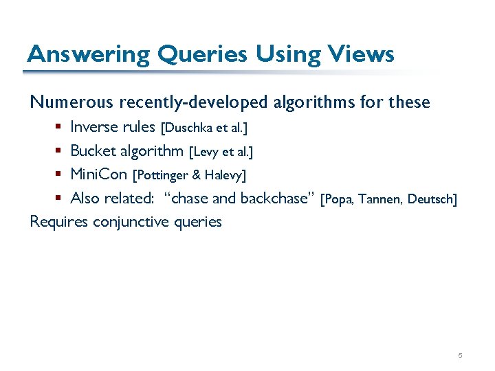
Answering Queries Using Views Numerous recently-developed algorithms for these § Inverse rules [Duschka et al. ] § Bucket algorithm [Levy et al. ] § Mini. Con [Pottinger & Halevy] § Also related: “chase and backchase” [Popa, Tannen, Deutsch] Requires conjunctive queries 5

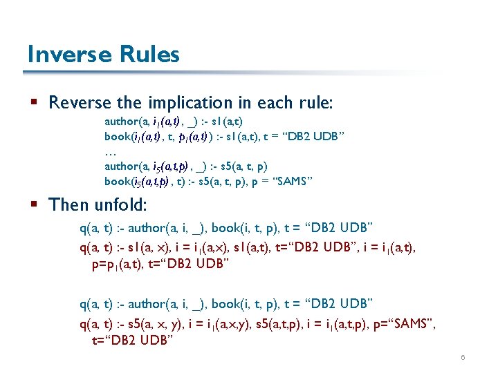
Inverse Rules § Reverse the implication in each rule: author(a, i 1(a, t), _) : - s 1(a, t) book(i 1(a, t), t, p 1(a, t)) : - s 1(a, t), t = “DB 2 UDB” … author(a, i 5(a, t, p) , _) : - s 5(a, t, p) book(i 5(a, t, p) , t) : - s 5(a, t, p), p = “SAMS” § Then unfold: q(a, t) : - author(a, i, _), book(i, t, p), t = “DB 2 UDB” q(a, t) : - s 1(a, x), i = i 1(a, x), s 1(a, t), t=“DB 2 UDB”, i = i 1(a, t), p=p 1(a, t), t=“DB 2 UDB” q(a, t) : - author(a, i, _), book(i, t, p), t = “DB 2 UDB” q(a, t) : - s 5(a, x, y), i = i 1(a, x, y), s 5(a, t, p), i = i 1(a, t, p), p=“SAMS”, t=“DB 2 UDB” 6

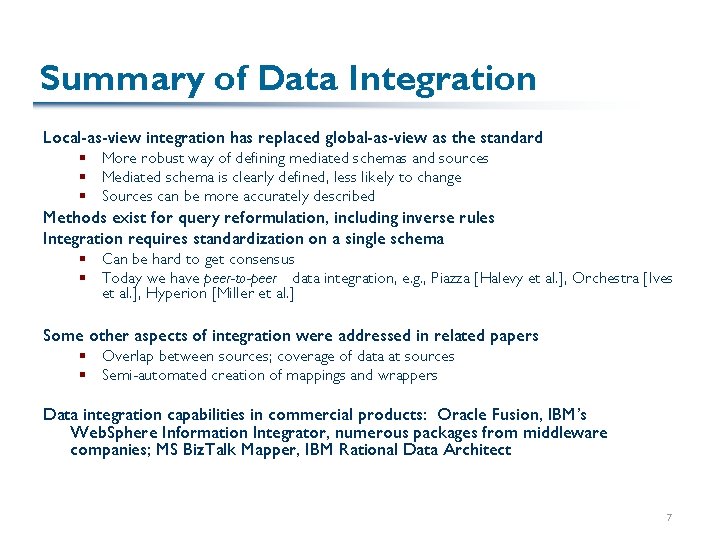
Summary of Data Integration Local-as-view integration has replaced global-as-view as the standard § More robust way of defining mediated schemas and sources § Mediated schema is clearly defined, less likely to change § Sources can be more accurately described Methods exist for query reformulation, including inverse rules Integration requires standardization on a single schema § Can be hard to get consensus § Today we have peer-to-peer data integration, e. g. , Piazza [Halevy et al. ], Orchestra [Ives et al. ], Hyperion [Miller et al. ] Some other aspects of integration were addressed in related papers § Overlap between sources; coverage of data at sources § Semi-automated creation of mappings and wrappers Data integration capabilities in commercial products: Oracle Fusion, IBM’s Web. Sphere Information Integrator, numerous packages from middleware companies; MS Biz. Talk Mapper, IBM Rational Data Architect 7

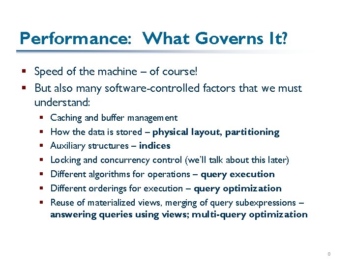
Performance: What Governs It? § Speed of the machine – of course! § But also many software-controlled factors that we must understand: § § § § Caching and buffer management How the data is stored – physical layout, partitioning Auxiliary structures – indices Locking and concurrency control (we’ll talk about this later) Different algorithms for operations – query execution Different orderings for execution – query optimization Reuse of materialized views, merging of query subexpressions – answering queries using views; multi-query optimization 8

Our General Emphasis § Goal: cover basic principles that are applied throughout database system design § Use the appropriate strategy in the appropriate place Every (reasonable) algorithm is good somewhere § … And a corollary: database people reinvent a lot of things and add minor tweaks… 9

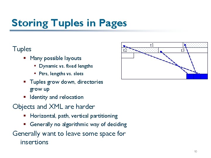
Storing Tuples in Pages t 1 Tuples t 2 t 3 § Many possible layouts Dynamic vs. fixed lengths Ptrs, lengths vs. slots § Tuples grow down, directories grow up § Identity and relocation Objects and XML are harder § Horizontal, path, vertical partitioning § Generally no algorithmic way of deciding Generally want to leave some space for insertions 10

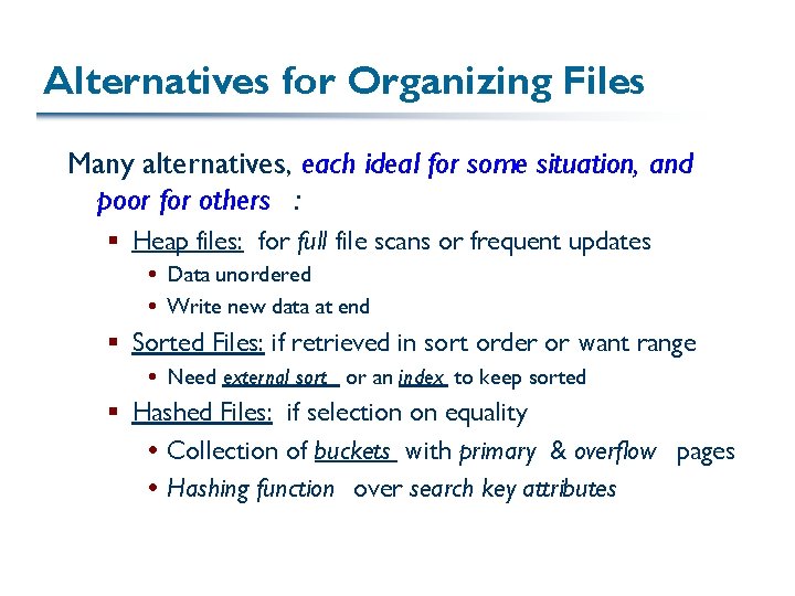
Alternatives for Organizing Files Many alternatives, each ideal for some situation, and poor for others : § Heap files: for full file scans or frequent updates Data unordered Write new data at end § Sorted Files: if retrieved in sort order or want range Need external sort or an index to keep sorted § Hashed Files: if selection on equality Collection of buckets with primary & overflow pages Hashing function over search key attributes

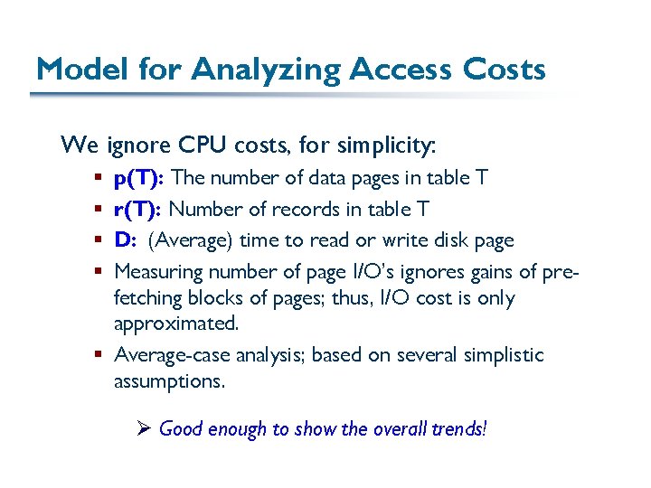
Model for Analyzing Access Costs We ignore CPU costs, for simplicity: p(T): The number of data pages in table T r(T): Number of records in table T D: (Average) time to read or write disk page Measuring number of page I/O’s ignores gains of prefetching blocks of pages; thus, I/O cost is only approximated. § Average-case analysis; based on several simplistic assumptions. § § Ø Good enough to show the overall trends!

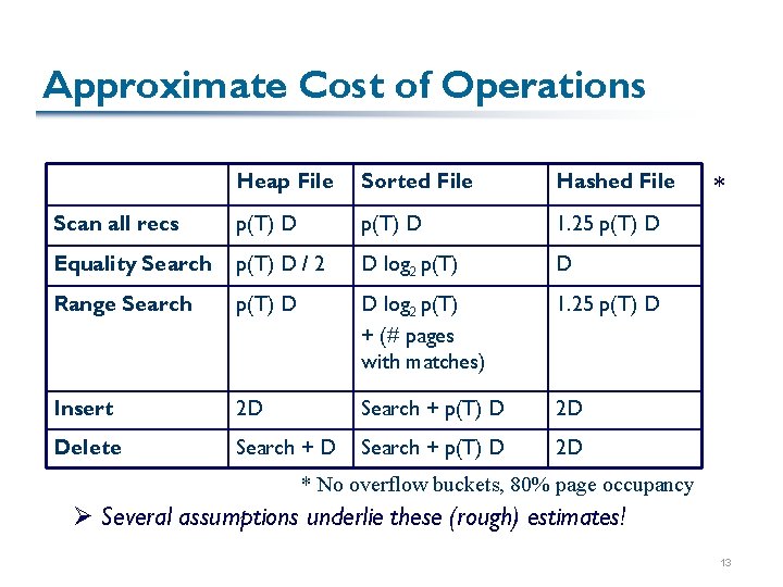
Approximate Cost of Operations Heap File Sorted File Hashed File Scan all recs p(T) D 1. 25 p(T) D Equality Search p(T) D / 2 D log 2 p(T) D Range Search p(T) D D log 2 p(T) + (# pages with matches) 1. 25 p(T) D Insert 2 D Search + p(T) D 2 D Delete Search + D Search + p(T) D 2 D * * No overflow buckets, 80% page occupancy Ø Several assumptions underlie these (rough) estimates! 13

Speeding Operations over Data § Recall that we’re interested in how to get good performance in answering queries § The first consideration is how the data is made accessible to the DBMS § We saw different arrangements of the tables: Heap (unsorted) files, sorted files, and hashed files § Today we look further at 3 core concepts that are used to efficiently support sort- and hash-based access to data: § Indexing § Sorting § Hashing 14

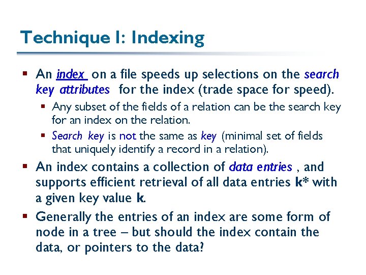
Technique I: Indexing § An index on a file speeds up selections on the search key attributes for the index (trade space for speed). § Any subset of the fields of a relation can be the search key for an index on the relation. § Search key is not the same as key (minimal set of fields that uniquely identify a record in a relation). § An index contains a collection of data entries , and supports efficient retrieval of all data entries k* with a given key value k. § Generally the entries of an index are some form of node in a tree – but should the index contain the data, or pointers to the data?

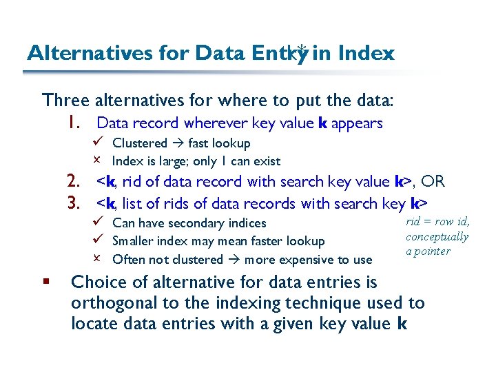
Alternatives for Data Entry k* in Index Three alternatives for where to put the data: 1. Data record wherever key value k appears ü Clustered fast lookup O Index is large; only 1 can exist 2. <k, rid of data record with search key value k>, OR 3. <k, list of rids of data records with search key k> ü Can have secondary indices ü Smaller index may mean faster lookup O Often not clustered more expensive to use § rid = row id, conceptually a pointer Choice of alternative for data entries is orthogonal to the indexing technique used to locate data entries with a given key value k

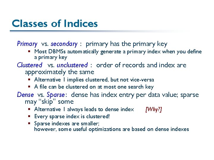
Classes of Indices Primary vs. secondary : primary has the primary key § Most DBMSs automatically generate a primary index when you define a primary key Clustered vs. unclustered : order of records and index are approximately the same § Alternative 1 implies clustered, but not vice-versa § A file can be clustered on at most one search key Dense vs. Sparse : dense has index entry per data value; sparse may “skip” some § Alternative 1 always leads to dense index [Why? ] § Every sparse index is clustered! § Sparse indexes are smaller; however, some useful optimizations are based on dense indexes

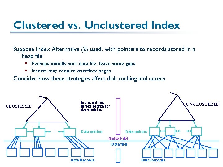
Clustered vs. Unclustered Index Suppose Index Alternative (2) used, with pointers to records stored in a heap file § Perhaps initially sort data file, leave some gaps § Inserts may require overflow pages Consider how these strategies affect disk caching and access CLUSTERED Index entries direct search for data entries Data entries UNCLUSTERED Data entries (Index File) (Data file) Data Records

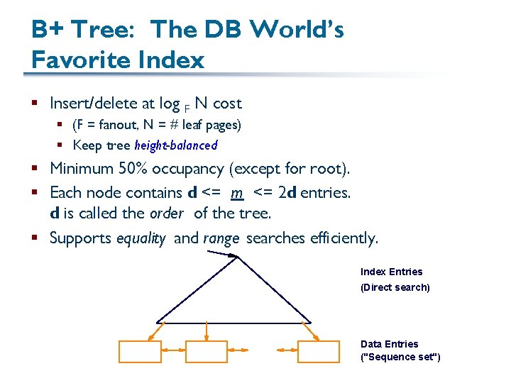
B+ Tree: The DB World’s Favorite Index § Insert/delete at log F N cost § (F = fanout, N = # leaf pages) § Keep tree height-balanced § Minimum 50% occupancy (except for root). § Each node contains d <= m <= 2 d entries. d is called the order of the tree. § Supports equality and range searches efficiently. Index Entries (Direct search) Data Entries ("Sequence set")

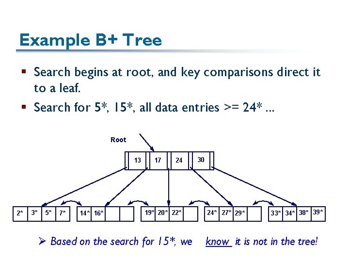
Example B+ Tree § Search begins at root, and key comparisons direct it to a leaf. § Search for 5*, 15*, all data entries >= 24*. . . Root 13 2* 3* 5* 7* 14* 16* 17 24 19* 20* 22* Ø Based on the search for 15*, we 30 24* 27* 29* 33* 34* 38* 39* know it is not in the tree!

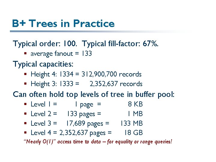
B+ Trees in Practice Typical order: 100. Typical fill-factor: 67%. § average fanout = 133 Typical capacities: § Height 4: 1334 = 312, 900, 700 records § Height 3: 1333 = 2, 352, 637 records Can often hold top levels of tree in buffer pool: § § Level 1 = 1 page = Level 2 = 133 pages = Level 3 = 17, 689 pages = Level 4 = 2, 352, 637 pages = 8 KB 1 MB 133 MB 18 GB “Nearly O(1)” access time to data – for equality or range queries!

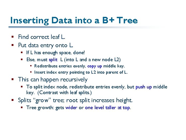
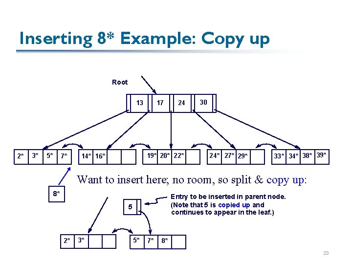
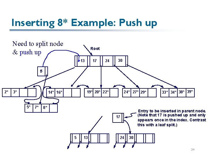
Inserting Data into a B+ Tree § Find correct leaf L. § Put data entry onto L. § If L has enough space, done! § Else, must split L (into L and a new node L 2) Redistribute entries evenly, copy up middle key. Insert index entry pointing to L 2 into parent of L. § This can happen recursively § To split index node, redistribute entries evenly, but push up middle key. (Contrast with leaf splits. ) § Splits “grow” tree; root split increases height. § Tree growth: gets wider or one level taller at top.

Inserting 8* Example: Copy up Root 13 2* 3* 5* 7* 17 24 19* 20* 22* 14* 16* 30 24* 27* 29* 33* 34* 38* 39* Want to insert here; no room, so split & copy up: 8* Entry to be inserted in parent node. (Note that 5 is copied up and continues to appear in the leaf. ) 5 2* 3* 5* 7* 8* 23

Inserting 8* Example: Push up Need to split node & push up Root 13 17 24 30 5 2* 3* 19* 20* 22* 14* 16* 5* 7* 24* 27* 29* 8* Entry to be inserted in parent node. (Note that 17 is pushed up and only appears once in the index. Contrast this with a leaf split. ) 17 5 13 24 33* 34* 38* 39* 30 24

Deleting Data from a B+ Tree § Start at root, find leaf L where entry belongs. § Remove the entry. § If L is at least half-full, done! § If L has only d-1 entries, Try to re-distribute, borrowing from sibling (adjacent node with same parent as L). If re-distribution fails, merge L and sibling. § If merge occurred, must delete entry (pointing to L or sibling) from parent of L. § Merge could propagate to root, decreasing height.

B+ Tree Summary B+ tree and other indices ideal for range searches, good for equality searches. § § § Inserts/deletes leave tree height-balanced; log. F N cost. High fanout (F) means depth rarely more than 3 or 4. Almost always better than maintaining a sorted file. Typically, 67% occupancy on average. Note: Order (d) concept replaced by physical space criterion in practice (“at least half-full”). Records may be variable sized Index pages typically hold more entries than leaves