CS 466666 Algorithm Design and Analysis Lecture 3

CS 466/666 Algorithm Design and Analysis Lecture 3 19 May 2020 1

Today’s Plan Finishing L 02 2 simple applications of Chernoff bound HW 1 posted, due June 1 Some sample projects posted Graph sparsification near linear time minimum cut algorithm? Dimension reduction 2

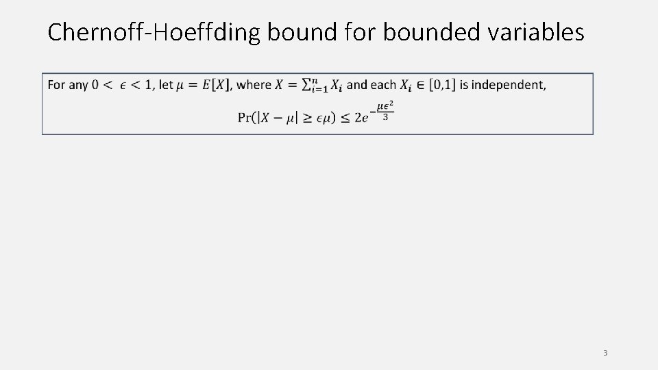
Chernoff-Hoeffding bound for bounded variables 3

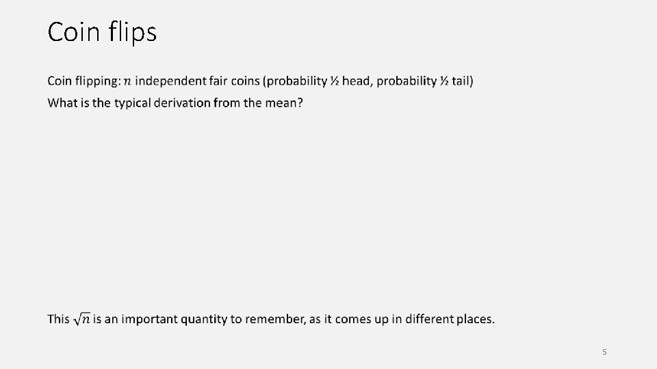
Coin flips 4

Coin flips 5

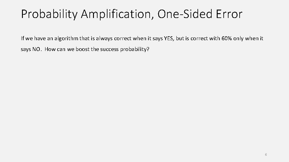
Probability Amplification, One-Sided Error If we have an algorithm that is always correct when it says YES, but is correct with 60% only when it says NO. How can we boost the success probability? 6

Probability Amplification, Two-Sided Error 7

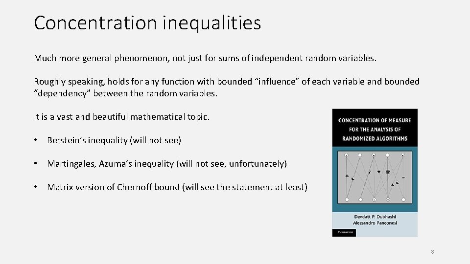
Concentration inequalities Much more general phenomenon, not just for sums of independent random variables. Roughly speaking, holds for any function with bounded “influence” of each variable and bounded “dependency” between the random variables. It is a vast and beautiful mathematical topic. • Berstein’s inequality (will not see) • Martingales, Azuma’s inequality (will not see, unfortunately) • Matrix version of Chernoff bound (will see the statement at least) 8

Homework Read chapter 3 and 4 of Mitzenmacher and Upfal. 9

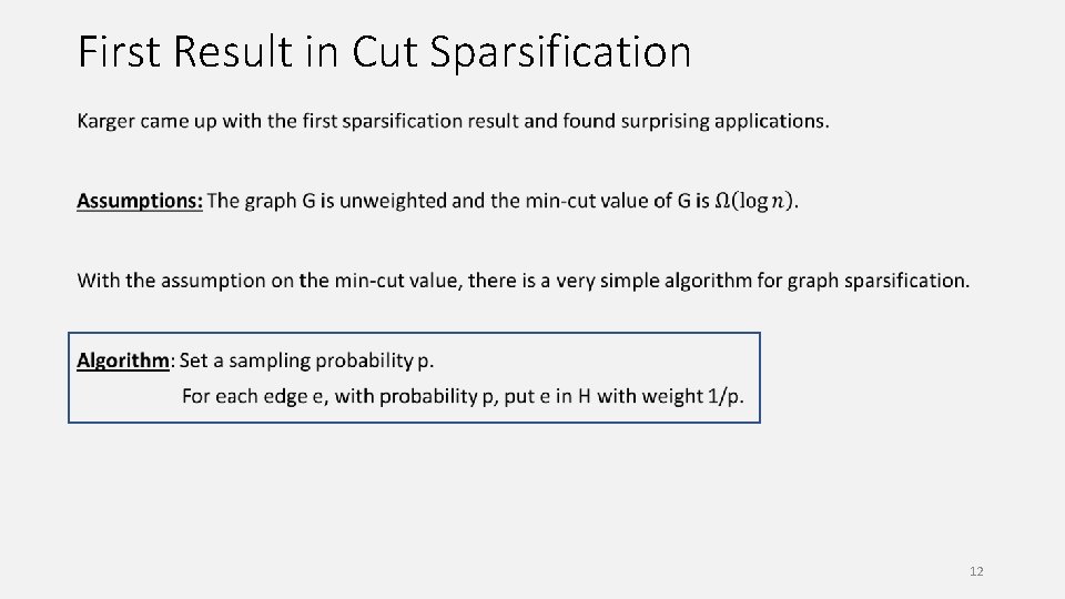
Graph Sparsification Given an undirected graph G=(V, E) with a weight w(e) on each edge e in E, we are interested in finding a “sparse” graph H that approximates G well. There are different notions of a sparsifier, depending on what properties to preserve. We study a notion called cut sparsifier. 10

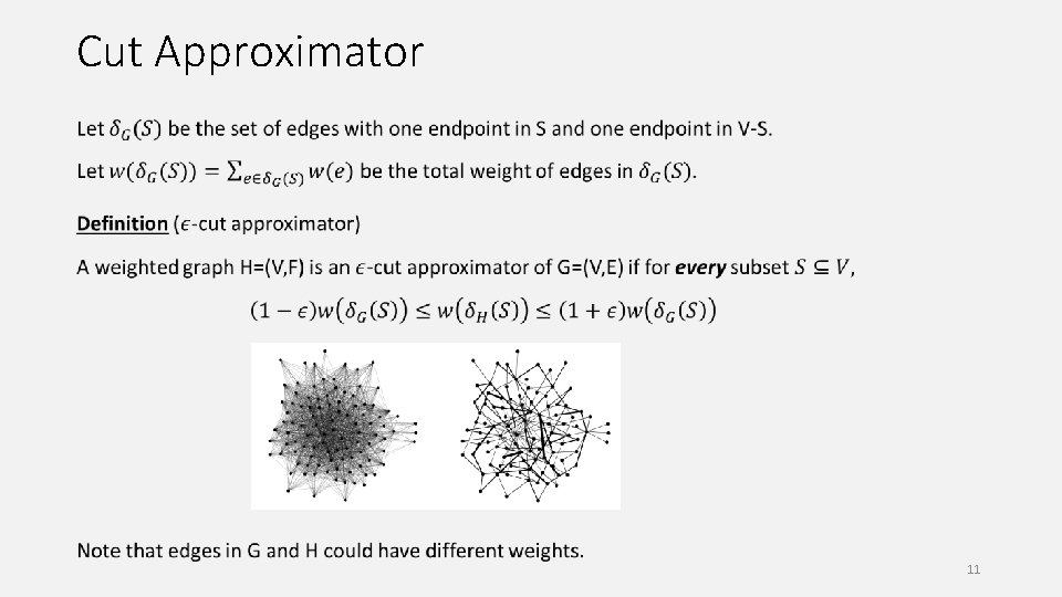
Cut Approximator 11

First Result in Cut Sparsification 12

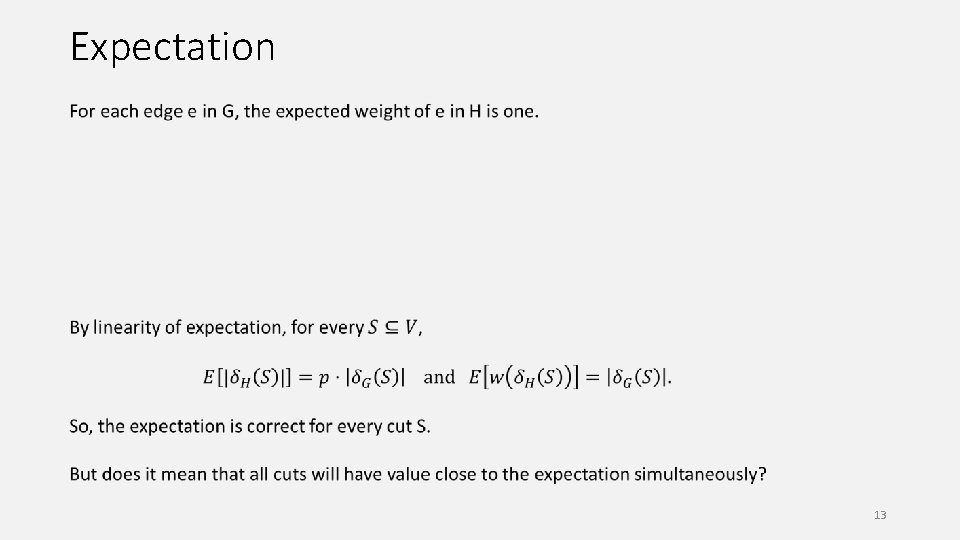
Expectation 13

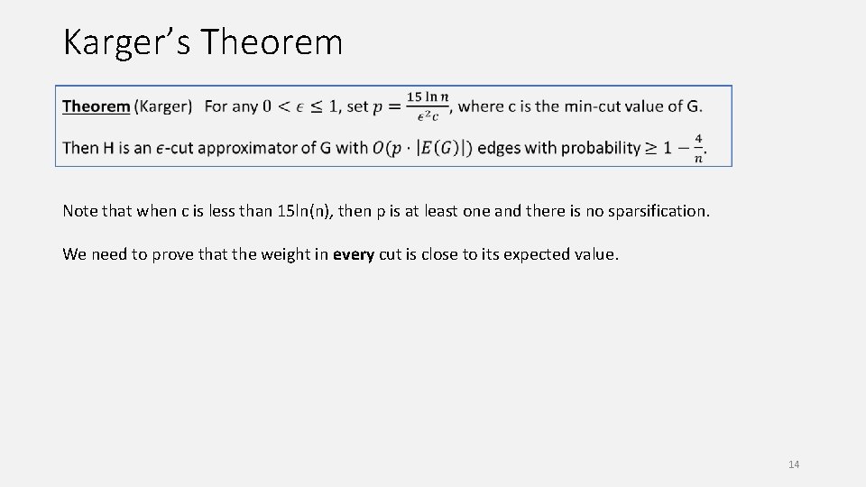
Karger’s Theorem Note that when c is less than 15 ln(n), then p is at least one and there is no sparsification. We need to prove that the weight in every cut is close to its expected value. 14

Analysis of One Cut 15

Simple union bound won’t work 16

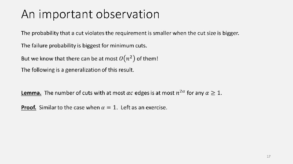
An important observation 17

A more careful union bound would work 18

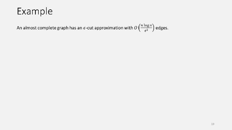
Example 19

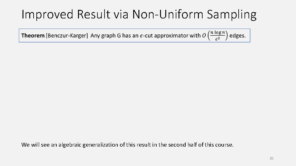
Improved Result via Non-Uniform Sampling We will see an algebraic generalization of this result in the second half of this course. 20

Standard Applications Design a fast approximation algorithm for the minimum s-t cut problem. 21

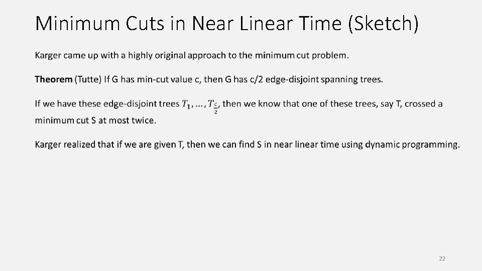
Minimum Cuts in Near Linear Time (Sketch) 22

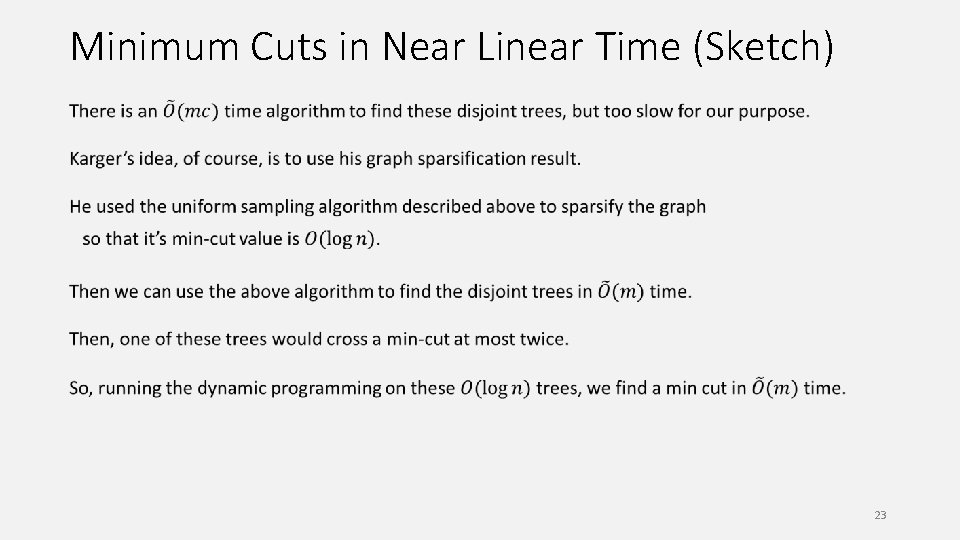
Minimum Cuts in Near Linear Time (Sketch) 23

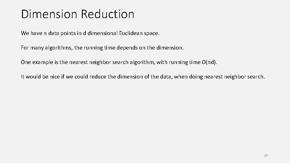
Dimension Reduction We have n data points in d dimensional Euclidean space. For many algorithms, the running time depends on the dimension. One example is the nearest neighbor search algorithm, with running time O(nd). It would be nice if we could reduce the dimension of the data, when doing nearest neighbor search. 24

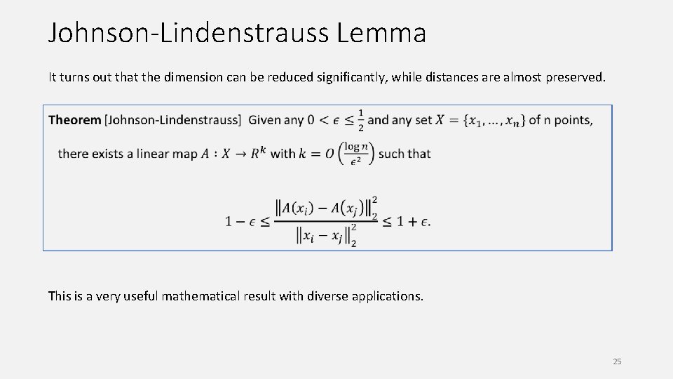
Johnson-Lindenstrauss Lemma It turns out that the dimension can be reduced significantly, while distances are almost preserved. This is a very useful mathematical result with diverse applications. 25

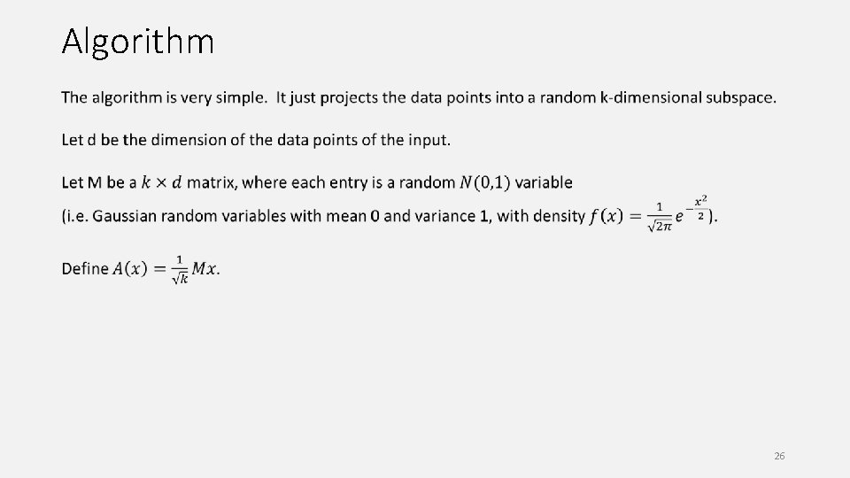
Algorithm 26

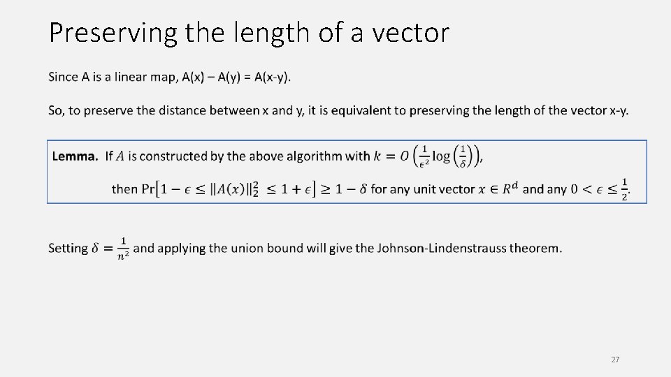
Preserving the length of a vector 27

Proof Idea 28

Two differences 1. For general x, each entry of Mx is still a N(0, 1) random variable. 2. We need to derive a Chernoff bound for sum of squares of independent Gaussians. 29

Applications 1. Approximate nearest neighbor search. 2. Approximate matrix multiplication. 30

Summary We have seen two interesting and important applications of concentration inequalities. Both are about reducing the input size while preserving some properties of interest. They are both useful in designing fast approximation algorithms. Chernoff bound plus union bound is already quite powerful. 31

Project Ideas 1. Concentration inequalities for analysis of randomized algorithms (e. g. martingale). 2. Graph sparsification and applications. 3. Algorithms for minimum cuts. 4. Metric embedding. 5. Randomized numerical linear algebra. 32