CS 466666 Algorithm Design and Analysis Lecture 5

CS 466/666 - Algorithm Design and Analysis Lecture 5: Hashing Waterloo, 26 May 2020 1

Today’s Plan Hashing: the setup 10 late days for HW and proposal, use carefully. Random hash functions? TA office hour, Wed 11 am-12 pm, Fri 10 pm-11 pm Pairwise independent random variables Universal hash functions 2

Data Structure for Searching We would like to build a data structure to support the following operations: 1. Insert(x): insert element x into the data structure 2. Delete(x): delete element x from the data structure 3. Search(x): check if x is in the data structure, i. e. return yes or no. Consider the scenario where we would like to store n keys/elements from the set/universe {0, 1, …, m-1}. Think of m >> n. For example, m is the number of possible IP addresses, and n is the number of IP addresses visiting Waterloo each day. 3

Random Access Model We assume the following computational model, called the random access model (RAM): 1. We can access an arbitrary position of an array (no matter how large) in O(1) time. 2. Each element in the universe can be fit into one word, and each arithmetic operation involving a word takes O(1) time, e. g. addition/multiplication of two words. These assumptions are not necessarily realistic. So, when we say hashing can be done in O(1) time, it is more accurate to say that hashing can be done in O(1) array lookup operations and O(1) word operations. 4

Obvious Solution Consider the scenario where we would like to store n keys/elements from the set/universe {0, 1, …, m-1}. With the RAM assumptions, we can easily build a data structure for searching in O(1) time. • Open an array A of m elements, initially A[i]=0 for all i. • When we insert element x, we set A[x]=1. • When we delete element x, we set A[x]=0. • When we search element x, if A[x]=1 return YES, else if A[x]=0 return NO. With the RAM assumptions, clearly each operation can be done in O(1) time. 5

Ideal Solution What is the problem with this data structure? The space requirement is m bits. This is bad when m is much larger than n, e. g. m = # of possible IP addresses. We would like to have a data structure with O(n) space requirements and O(1) time per operation. 6

Hash Table: Deterministic Solution A hash function is used to map the elements in the big universe to the locations in a small table. A hash table consists of two components: 1. A table with n cells indexed by N={0, 1, …, n-1}, each cell can store O(log m) bits. 2. A hash function h: M->N. Ideally, we want the hash function h to map different keys to different cells. But, by the pigeonhole principle, this is impossible if we do not know the keys in advance. There is just no deterministic solution for hashing. 7

Hash Table: Randomized Solution A hash function is used to map the elements in the big universe to the locations in a small table. A hash table consists of two components: 1. A table with n cells indexed by N={0, 1, …, n-1}, each cell can store O(log m) bits. 2. A hash function h: M->N chosen randomly from a family H of hash functions. We assume the keys are independent of the hash function that we choose, i. e. there is no “adversary” who knows our internal randomness and choose a bad set of keys for our hash function. 8

Analysis of Randomized Algorithms The situation is the same when we analyze randomized algorithms. A randomized algorithm is just a family of deterministic algorithms, one for each possible random string. For some problems, there does not exist one single deterministic algorithm that is good for all inputs. Instead, we relax this requirement for a randomized algorithm to: for every input, there are say at least 90% of deterministic algorithms that are good for this input. In the case of hashing, we relax the requirement to: for every set of n keys, there are say at least 90% of hash functions h in the hash family H such that there are “few” keys that are mapped to the same cell. 9

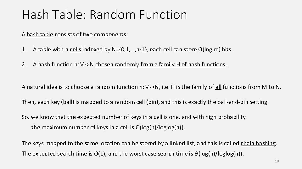
Hash Table: Random Function A hash table consists of two components: 1. A table with n cells indexed by N={0, 1, …, n-1}, each cell can store O(log m) bits. 2. A hash function h: M->N chosen randomly from a family H of hash functions. A natural idea is to choose a random function h: M->N, i. e. H is the family of all functions from M to N. Then, each key (ball) is mapped to a random cell (bin), and this is exactly the ball-and-bin setting. So, we know that the expected number of keys in a cell is one, and with high probability the maximum number of keys in a cell is Ɵ(log(n)/loglog(n)). The keys mapped to the same location can be stored by a linked list, and this is called chain hashing. The expected search time is O(1), and the worst case search time is Ɵ(log(n)/loglog(n)). 10

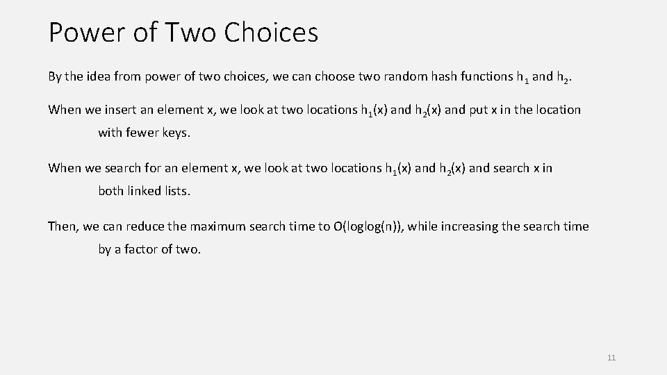
Power of Two Choices By the idea from power of two choices, we can choose two random hash functions h 1 and h 2. When we insert an element x, we look at two locations h 1(x) and h 2(x) and put x in the location with fewer keys. When we search for an element x, we look at two locations h 1(x) and h 2(x) and search x in both linked lists. Then, we can reduce the maximum search time to O(loglog(n)), while increasing the search time by a factor of two. 11

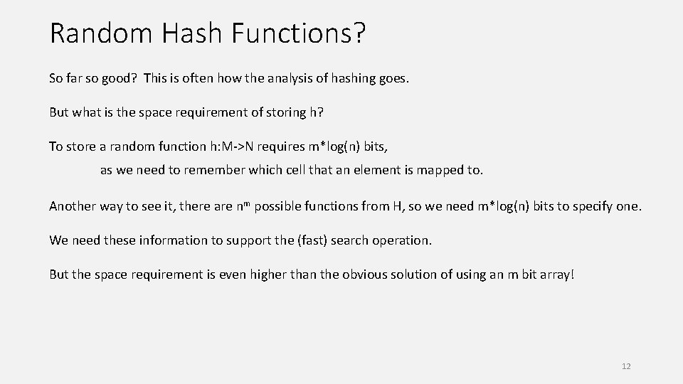
Random Hash Functions? So far so good? This is often how the analysis of hashing goes. But what is the space requirement of storing h? To store a random function h: M->N requires m*log(n) bits, as we need to remember which cell that an element is mapped to. Another way to see it, there are nm possible functions from H, so we need m*log(n) bits to specify one. We need these information to support the (fast) search operation. But the space requirement is even higher than the obvious solution of using an m bit array! 12

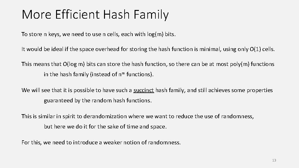
More Efficient Hash Family To store n keys, we need to use n cells, each with log(m) bits. It would be ideal if the space overhead for storing the hash function is minimal, using only O(1) cells. This means that O(log m) bits can store the hash function, so there can be at most poly(m) functions in the hash family (instead of nm functions). We will see that it is possible to have such a succinct hash family, and still achieves some properties guaranteed by the random hash functions. This is similar in spirit to derandomization where we want to reduce the use of randomness, but here we do it for the sake of time and space. For this, we need to introduce a weaker notion of randomness. 13

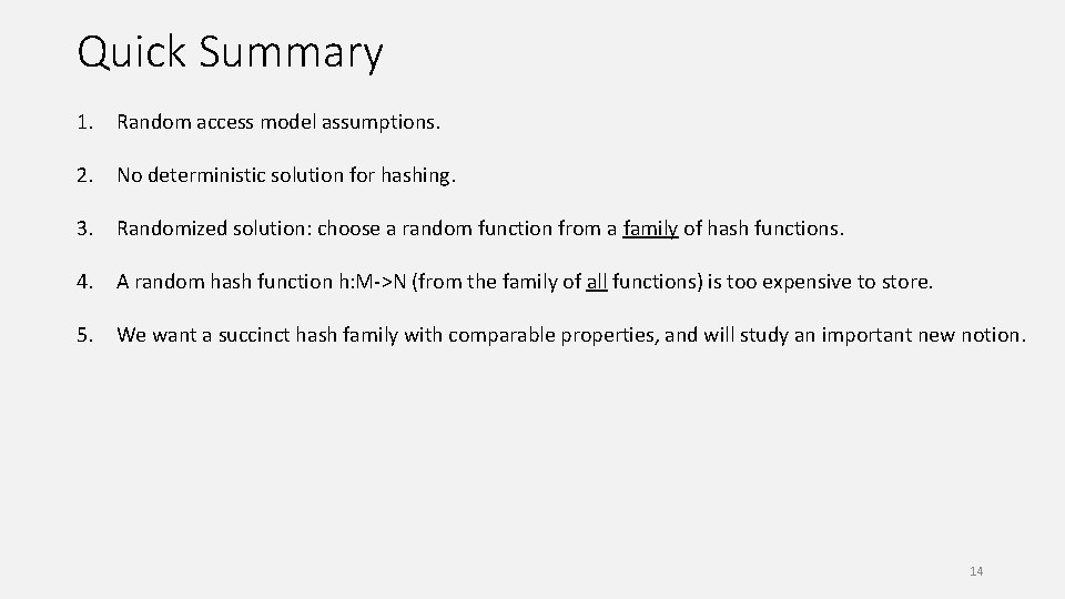
Quick Summary 1. Random access model assumptions. 2. No deterministic solution for hashing. 3. Randomized solution: choose a random function from a family of hash functions. 4. A random hash function h: M->N (from the family of all functions) is too expensive to store. 5. We want a succinct hash family with comparable properties, and will study an important new notion. 14

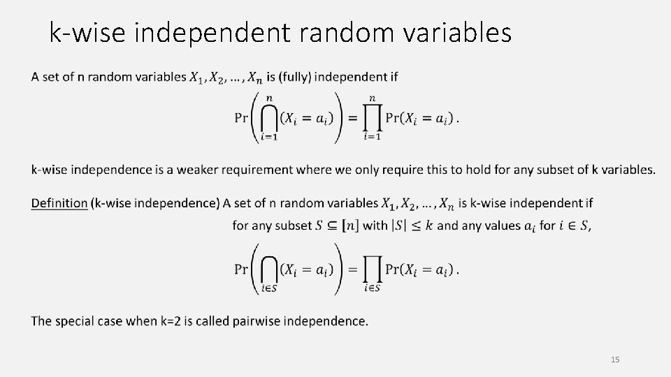
k-wise independent random variables 15

1 -wise independence is trivial What about 2 -wise independence? 16

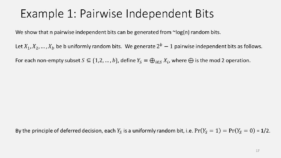
Example 1: Pairwise Independent Bits 17

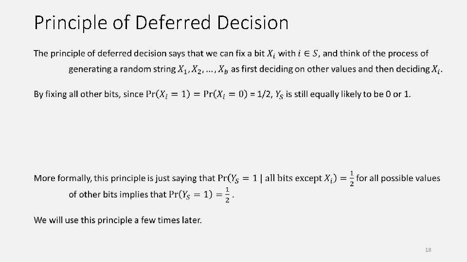
Principle of Deferred Decision 18

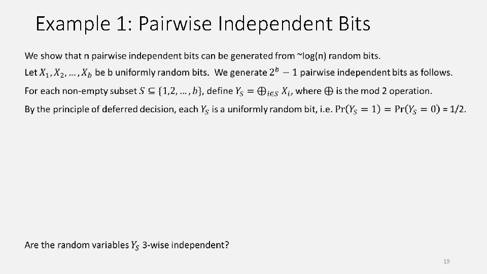
Example 1: Pairwise Independent Bits 19

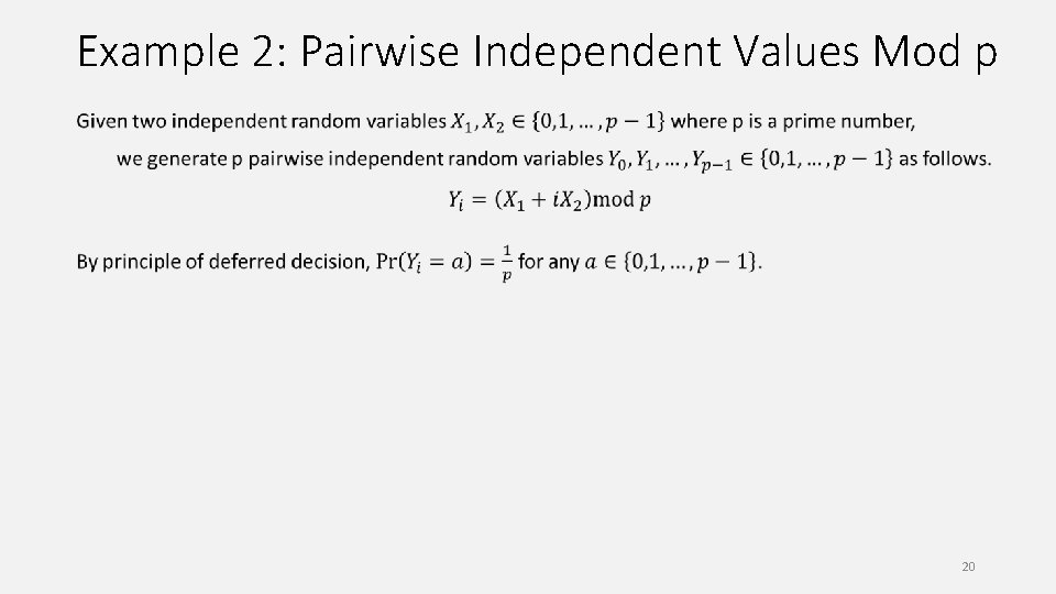
Example 2: Pairwise Independent Values Mod p 20

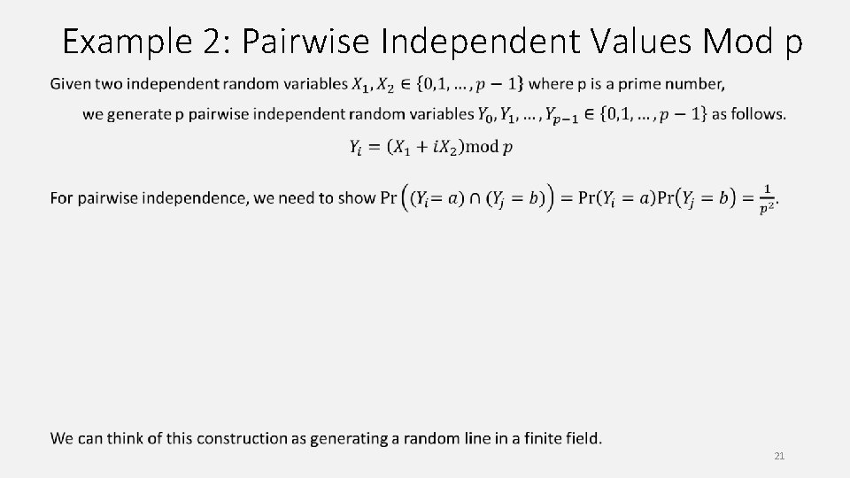
Example 2: Pairwise Independent Values Mod p 21

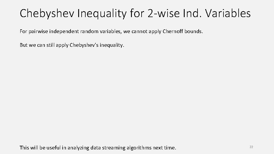
Chebyshev Inequality for 2 -wise Ind. Variables For pairwise independent random variables, we cannot apply Chernoff bounds. But we can still apply Chebyshev’s inequality. This will be useful in analyzing data streaming algorithms next time. 22

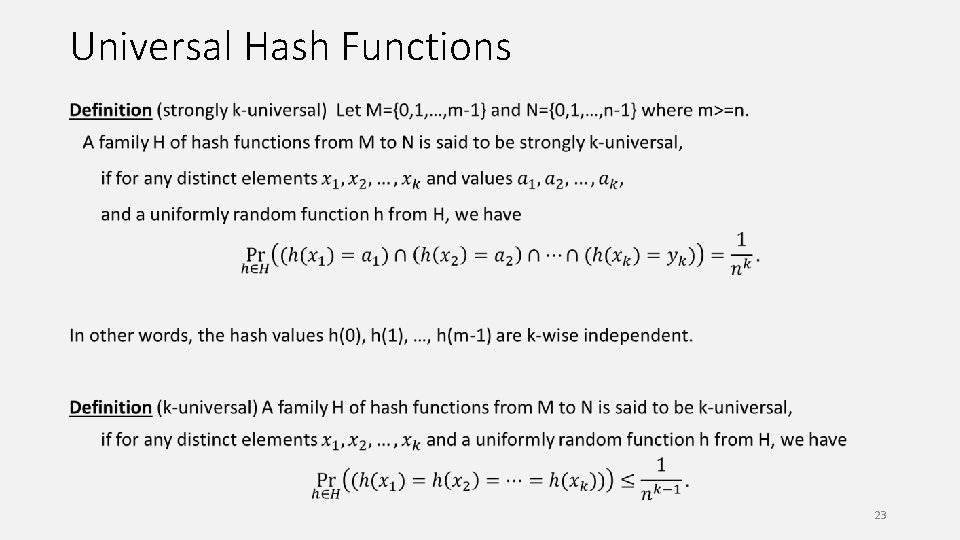
Universal Hash Functions 23

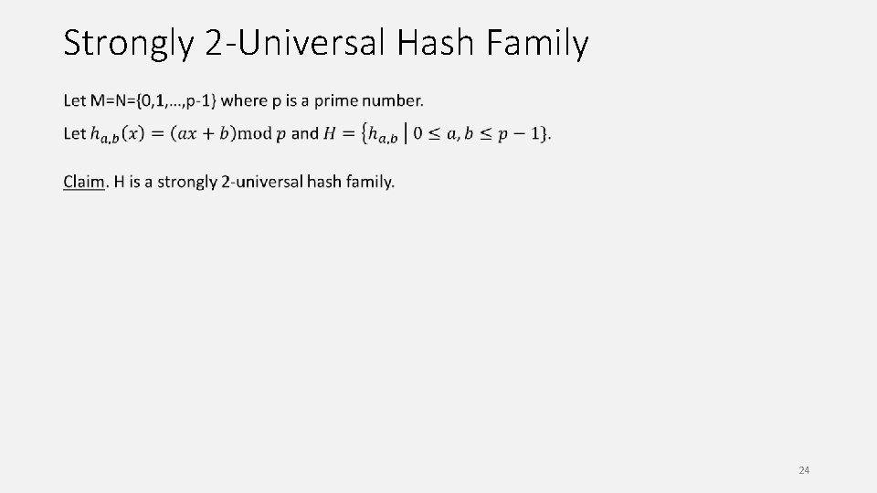
Strongly 2 -Universal Hash Family 24

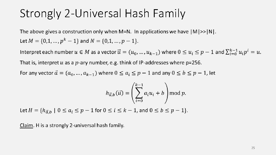
Strongly 2 -Universal Hash Family 25

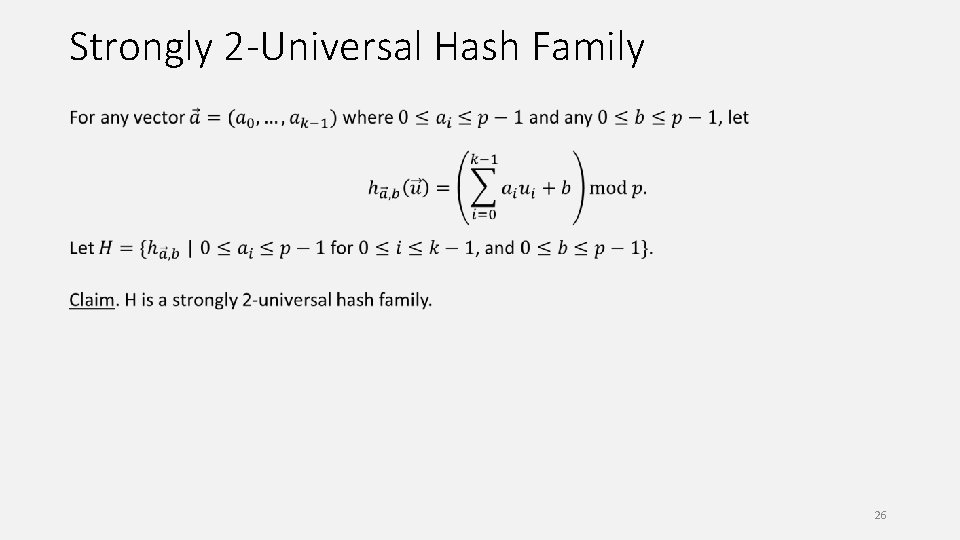
Strongly 2 -Universal Hash Family 26

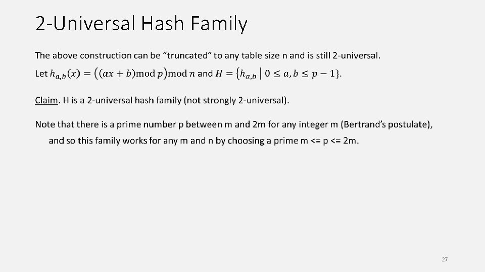
2 -Universal Hash Family 27

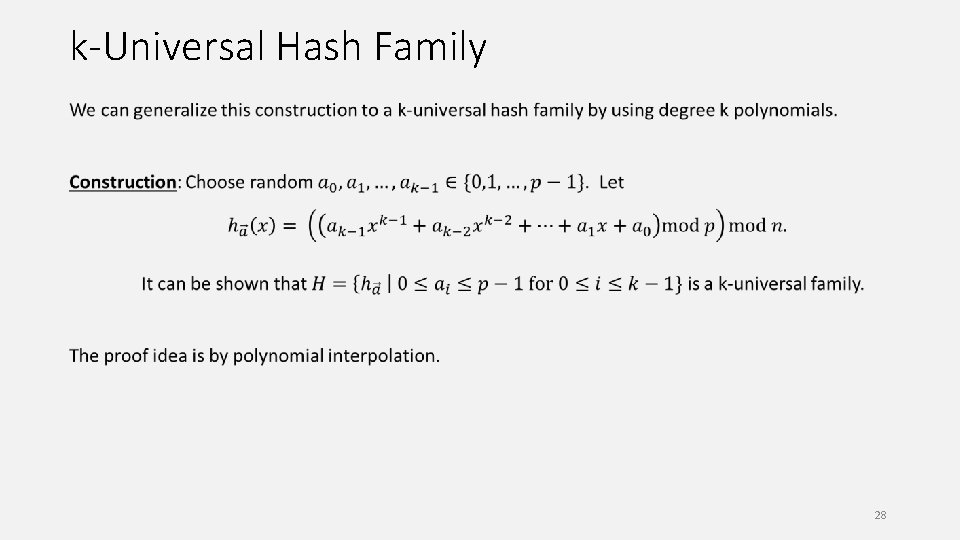
k-Universal Hash Family 28

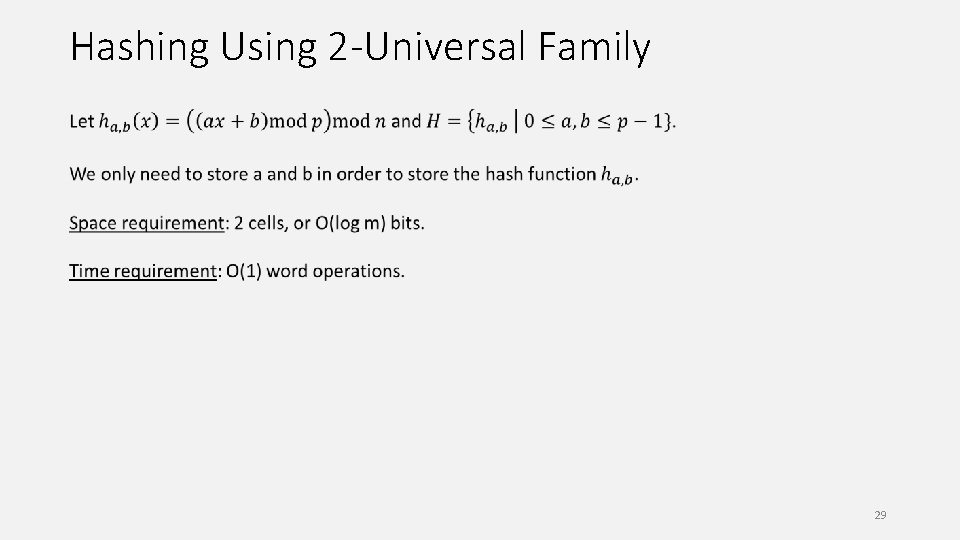
Hashing Using 2 -Universal Family 29

Expected Search Time 30

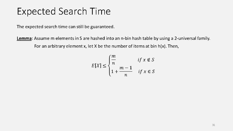
Expected Search Time 31

Maximum Load We cannot guarantee that the maximum load is O(log(n)/loglog(n)) anymore. We say a pair of elements i, j is a collision pair if i≠j but h(i)=h(j). 32

Maximum Load We cannot guarantee that the maximum load is O(log(n)/loglog(n)) anymore. To guarantee that the maximum load is O(log(n)/loglog(n)), we say use a O(log(n)/loglog(n))-universal hash family (why? ). But this is not a good tradeoff. 33

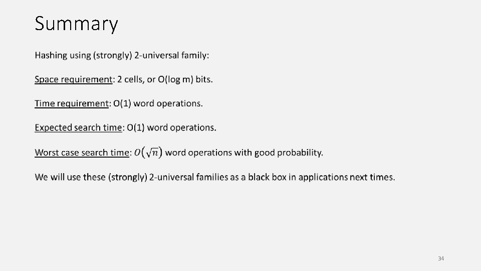
Summary 34