CS 152 Computer Architecture and Engineering Lecture 3

CS 152 Computer Architecture and Engineering Lecture 3 Performance, Technology & Delay Modeling CS 152 Lec 3. 1

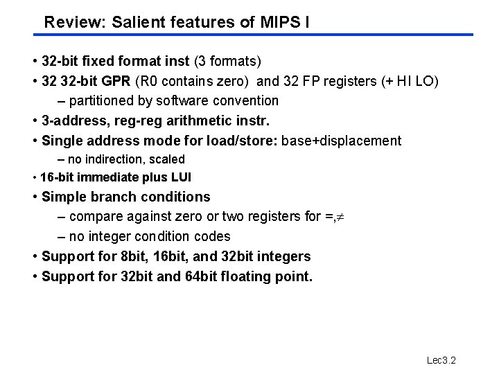
Review: Salient features of MIPS I • 32 -bit fixed format inst (3 formats) • 32 32 -bit GPR (R 0 contains zero) and 32 FP registers (+ HI LO) – partitioned by software convention • 3 -address, reg-reg arithmetic instr. • Single address mode for load/store: base+displacement – no indirection, scaled • 16 -bit immediate plus LUI • Simple branch conditions – compare against zero or two registers for =, – no integer condition codes • Support for 8 bit, 16 bit, and 32 bit integers • Support for 32 bit and 64 bit floating point. Lec 3. 2

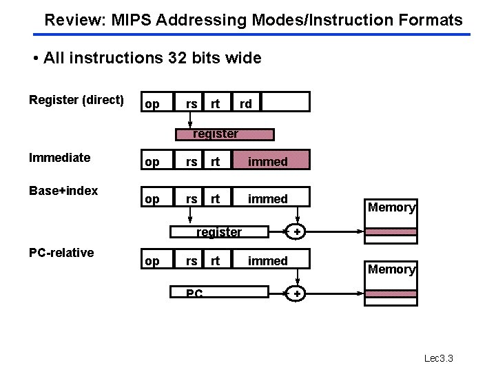
Review: MIPS Addressing Modes/Instruction Formats • All instructions 32 bits wide Register (direct) op rs rt rd register Immediate Base+index op rs rt immed register PC-relative op rs PC rt Memory + immed Memory + Lec 3. 3

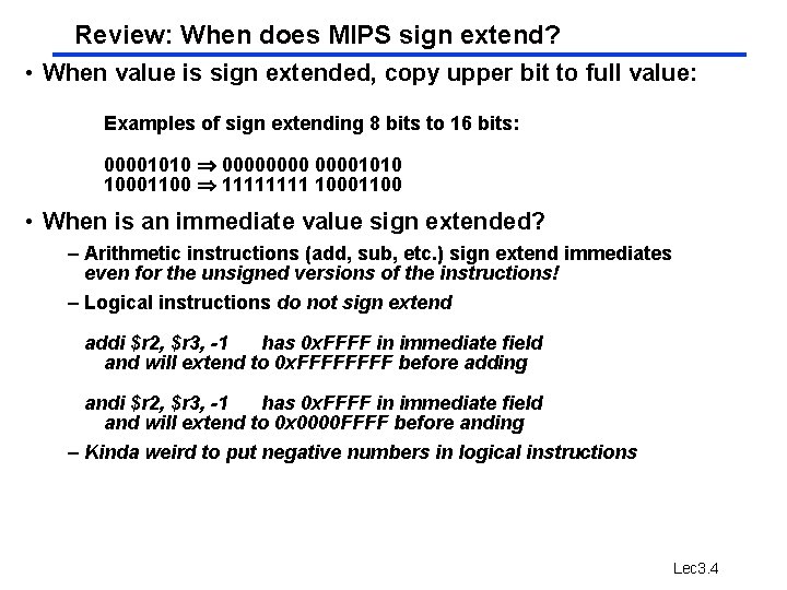
Review: When does MIPS sign extend? • When value is sign extended, copy upper bit to full value: Examples of sign extending 8 bits to 16 bits: 00001010 00001010 10001100 1111 10001100 • When is an immediate value sign extended? – Arithmetic instructions (add, sub, etc. ) sign extend immediates even for the unsigned versions of the instructions! – Logical instructions do not sign extend addi $r 2, $r 3, -1 has 0 x. FFFF in immediate field and will extend to 0 x. FFFF before adding andi $r 2, $r 3, -1 has 0 x. FFFF in immediate field and will extend to 0 x 0000 FFFF before anding – Kinda weird to put negative numbers in logical instructions Lec 3. 4

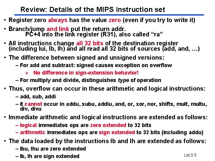
Review: Details of the MIPS instruction set • Register zero always has the value zero (even if you try to write it) • Branch/jump and link put the return addr. PC+4 into the link register (R 31), also called “ra” • All instructions change all 32 bits of the destination register (including lui, lb, lh) and all read all 32 bits of sources (add, and, …) • The difference between signed and unsigned versions: – For add and subtract: signed causes exception on overflow » No difference in sign-extension behavior! – For multiply and divide, distinguishes type of operation • Thus, overflow can occur in these arithmetic and logical instructions: – add, sub, addi – it cannot occur in addu, subu, addiu, and, or, xor, nor, shifts, multu, divu • Immediate arithmetic and logical instructions are extended as follows: – logical immediates ops are zero extended to 32 bits – arithmetic immediates ops are sign extended to 32 bits (including addu) • The data loaded by the instructions lb and lh are extended as follows: – lbu, lhu are zero extended – lb, lh are sign extended Lec 3. 5

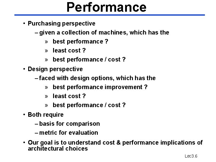
Performance • Purchasing perspective – given a collection of machines, which has the » best performance ? » least cost ? » best performance / cost ? • Design perspective – faced with design options, which has the » best performance improvement ? » least cost ? » best performance / cost ? • Both require – basis for comparison – metric for evaluation • Our goal is to understand cost & performance implications of architectural choices Lec 3. 6

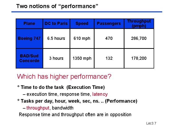
Two notions of “performance” Plane DC to Paris Speed Passengers Throughput (pmph) Boeing 747 6. 5 hours 610 mph 470 286, 700 BAD/Sud Concorde 3 hours 1350 mph 132 178, 200 Which has higher performance? ° Time to do the task (Execution Time) – execution time, response time, latency ° Tasks per day, hour, week, sec, ns. . . (Performance) – throughput, bandwidth Response time and throughput often are in opposition Lec 3. 7

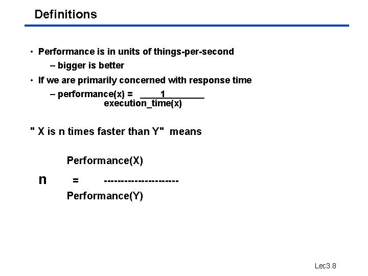
Definitions • Performance is in units of things-per-second – bigger is better • If we are primarily concerned with response time – performance(x) = 1 execution_time(x) " X is n times faster than Y" means Performance(X) n = ----------- Performance(Y) Lec 3. 8

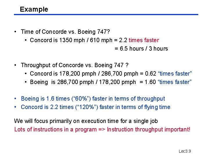
Example • Time of Concorde vs. Boeing 747? • Concord is 1350 mph / 610 mph = 2. 2 times faster = 6. 5 hours / 3 hours • Throughput of Concorde vs. Boeing 747 ? • Concord is 178, 200 pmph / 286, 700 pmph = 0. 62 “times faster” • Boeing is 286, 700 pmph / 178, 200 pmph = 1. 60 “times faster” • Boeing is 1. 6 times (“ 60%”) faster in terms of throughput • Concord is 2. 2 times (“ 120%”) faster in terms of flying time We will focus primarily on execution time for a single job Lots of instructions in a program => Instruction throughput important! Lec 3. 9

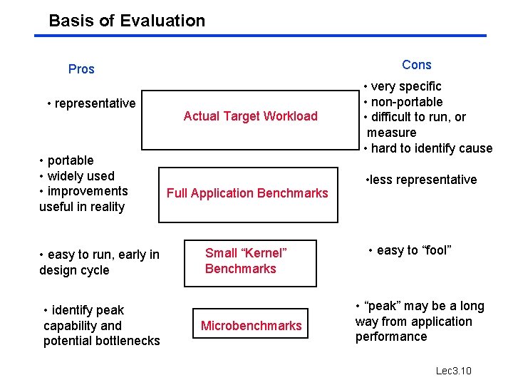
Basis of Evaluation Cons Pros • representative • portable • widely used • improvements useful in reality • easy to run, early in design cycle • identify peak capability and potential bottlenecks Actual Target Workload Full Application Benchmarks Small “Kernel” Benchmarks Microbenchmarks • very specific • non-portable • difficult to run, or measure • hard to identify cause • less representative • easy to “fool” • “peak” may be a long way from application performance Lec 3. 10

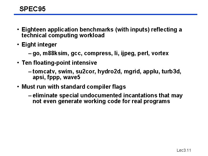
SPEC 95 • Eighteen application benchmarks (with inputs) reflecting a technical computing workload • Eight integer – go, m 88 ksim, gcc, compress, li, ijpeg, perl, vortex • Ten floating-point intensive – tomcatv, swim, su 2 cor, hydro 2 d, mgrid, applu, turb 3 d, apsi, fppp, wave 5 • Must run with standard compiler flags – eliminate special undocumented incantations that may not even generate working code for real programs Lec 3. 11

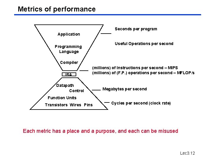
Metrics of performance Seconds per program Application Useful Operations per second Programming Language Compiler ISA (millions) of Instructions per second – MIPS (millions) of (F. P. ) operations per second – MFLOP/s Datapath Control Megabytes per second Function Units Transistors Wires Pins Cycles per second (clock rate) Each metric has a place and a purpose, and each can be misused Lec 3. 12

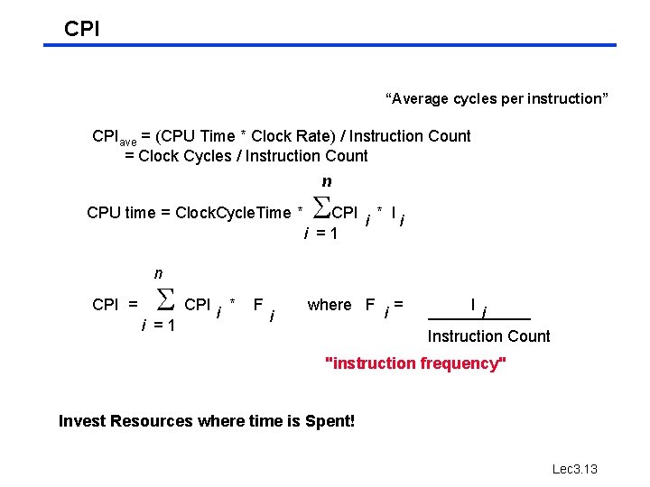
CPI “Average cycles per instruction” CPIave = (CPU Time * Clock Rate) / Instruction Count = Clock Cycles / Instruction Count n CPU time = Clock. Cycle. Time * CPI i * I i i =1 n CPI = CPI i * i =1 F i where F i = I i Instruction Count "instruction frequency" Invest Resources where time is Spent! Lec 3. 13

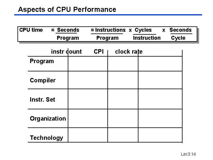
Aspects of CPU Performance CPU time = Seconds Program instr count = Instructions x Cycles Program CPI Instruction x Seconds Cycle clock rate Program Compiler Instr. Set Organization Technology Lec 3. 14

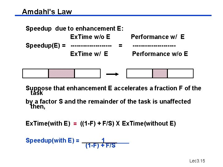
Amdahl's Law Speedup due to enhancement E: Ex. Time w/o E Speedup(E) = ---------- = Ex. Time w/ E Performance w/ E ----------Performance w/o E Suppose that enhancement E accelerates a fraction F of the task by a factor S and the remainder of the task is unaffected then, Ex. Time(with E) = ((1 -F) + F/S) X Ex. Time(without E) Speedup(with E) = 1 (1 -F) + F/S Lec 3. 15

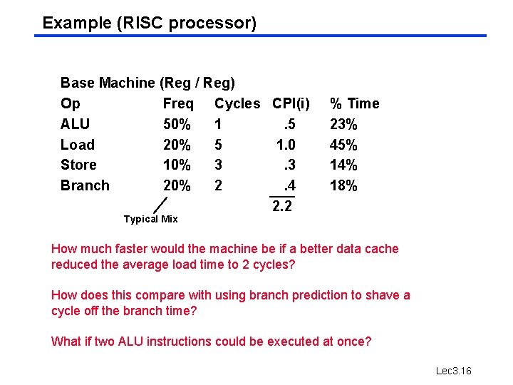
Example (RISC processor) Base Machine (Reg / Reg) Op Freq Cycles CPI(i) ALU 50% 1. 5 Load 20% 5 1. 0 Store 10% 3. 3 Branch 20% 2. 4 2. 2 % Time 23% 45% 14% 18% Typical Mix How much faster would the machine be if a better data cache reduced the average load time to 2 cycles? How does this compare with using branch prediction to shave a cycle off the branch time? What if two ALU instructions could be executed at once? Lec 3. 16

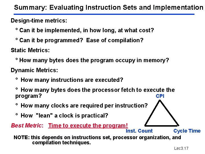
Summary: Evaluating Instruction Sets and Implementation Design-time metrics: ° Can it be implemented, in how long, at what cost? ° Can it be programmed? Ease of compilation? Static Metrics: ° How many bytes does the program occupy in memory? Dynamic Metrics: ° How many instructions are executed? ° How many bytes does the processor fetch to execute the program? CPI ° How many clocks are required per instruction? ° How "lean" a clock is practical? Best Metric: Time to execute the program! Inst. Count Cycle Time NOTE: this depends on instructions set, processor organization, and compilation techniques. Lec 3. 17

Administrative Matters Lec 3. 18

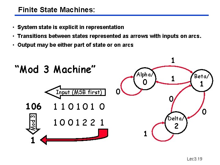
Finite State Machines: • System state is explicit in representation • Transitions between states represented as arrows with inputs on arcs. • Output may be either part of state or on arcs 1 “Mod 3 Machine” Input (MSB first) Mod 3 106 1 Alpha/ 0 0 1 Beta/ 1 0 1 1 0101 0 Delta/ 100122 1 1 0 2 Lec 3. 19

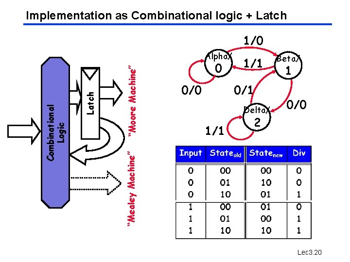
Implementation as Combinational logic + Latch 1/0 “Moore Machine” 0 0/0 1/1 0/1 Delta/ 1/1 Beta/ 1 0/0 2 “Mealey Machine” Latch Combinational Logic Alpha/ Lec 3. 20

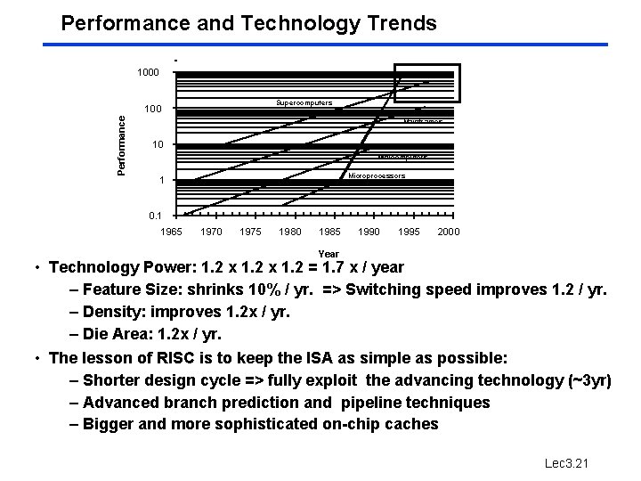
Performance and Technology Trends 1000 Supercomputers Performance 100 Mainframes 10 Minicomputers Microprocessors 1 0. 1 1965 1970 1975 1980 1985 1990 1995 2000 Year • Technology Power: 1. 2 x 1. 2 = 1. 7 x / year – Feature Size: shrinks 10% / yr. => Switching speed improves 1. 2 / yr. – Density: improves 1. 2 x / yr. – Die Area: 1. 2 x / yr. • The lesson of RISC is to keep the ISA as simple as possible: – Shorter design cycle => fully exploit the advancing technology (~3 yr) – Advanced branch prediction and pipeline techniques – Bigger and more sophisticated on-chip caches Lec 3. 21

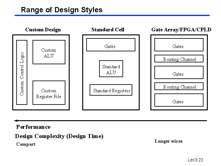
Range of Design Styles Custom Control Logic Custom Design Standard Cell Gates Custom ALU Standard Registers Performance Design Complexity (Design Time) Compact Gates Routing Channel Standard ALU Custom Register File Gate Array/FPGA/CPLD Gates Routing Channel Gates Longer wires Lec 3. 22

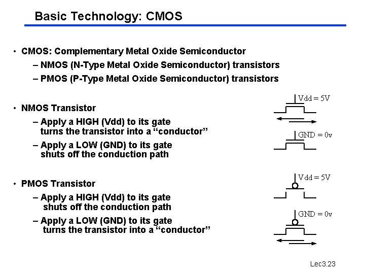
Basic Technology: CMOS • CMOS: Complementary Metal Oxide Semiconductor – NMOS (N-Type Metal Oxide Semiconductor) transistors – PMOS (P-Type Metal Oxide Semiconductor) transistors Vdd = 5 V • NMOS Transistor – Apply a HIGH (Vdd) to its gate turns the transistor into a “conductor” – Apply a LOW (GND) to its gate shuts off the conduction path • PMOS Transistor – Apply a HIGH (Vdd) to its gate shuts off the conduction path – Apply a LOW (GND) to its gate turns the transistor into a “conductor” GND = 0 v Vdd = 5 V GND = 0 v Lec 3. 23

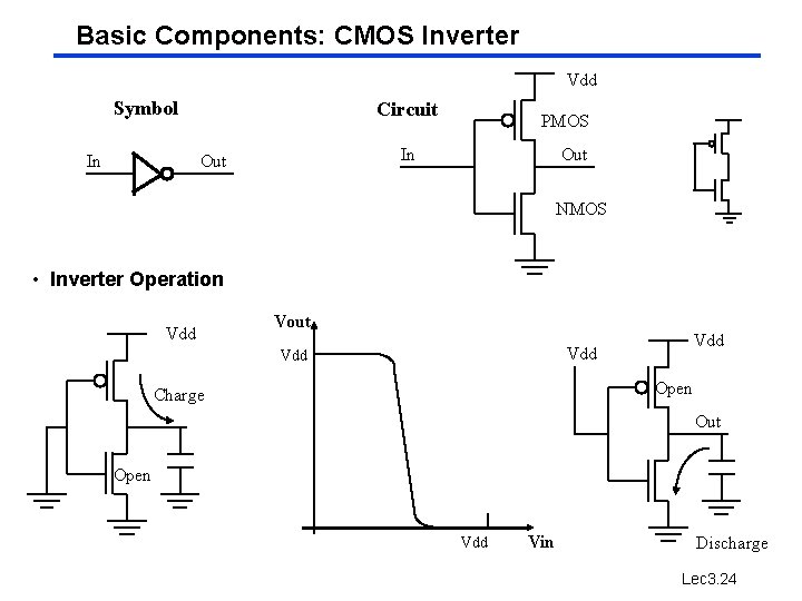
Basic Components: CMOS Inverter Vdd Symbol In Circuit PMOS In Out NMOS • Inverter Operation Vdd Vout Vdd Vdd Open Charge Out Open Vdd Vin Discharge Lec 3. 24

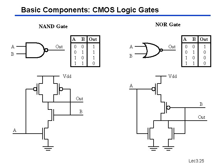
Basic Components: CMOS Logic Gates NOR Gate NAND Gate A A B Out 0 0 1 1 0 A A Out B Vdd 0 0 1 1 B Out 0 1 1 0 0 0 Vdd A Out B B Out A Lec 3. 25

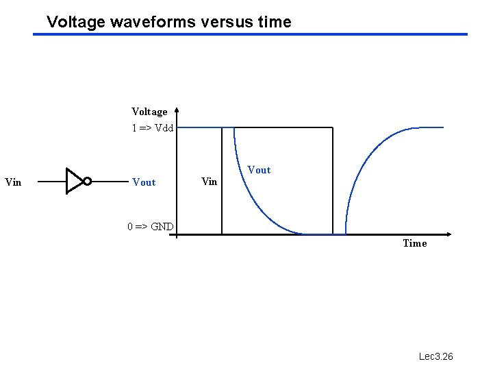
Voltage waveforms versus time Voltage 1 => Vdd Vin Vout 0 => GND Time Lec 3. 26

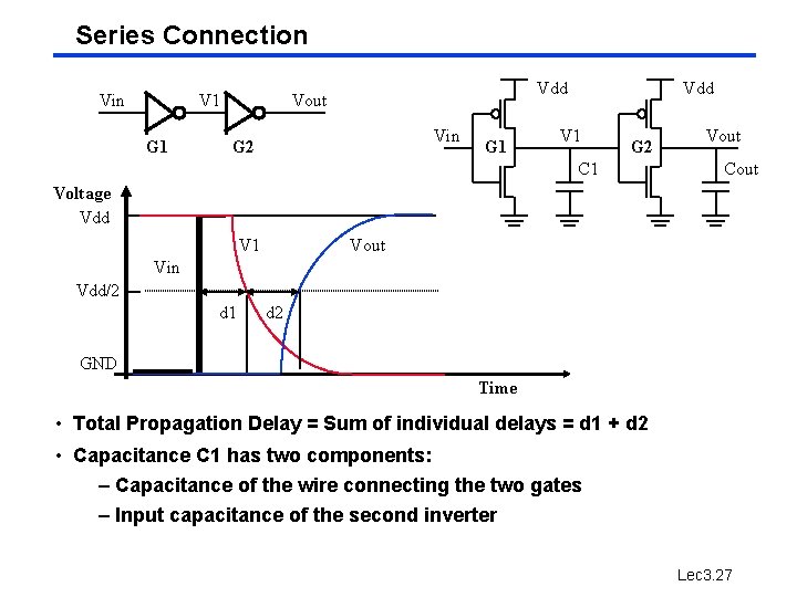
Series Connection Vin V 1 G 1 Vdd Vout Vin G 2 G 1 Vdd V 1 G 2 C 1 Vout Cout Voltage Vdd V 1 Vout Vin Vdd/2 d 1 d 2 GND Time • Total Propagation Delay = Sum of individual delays = d 1 + d 2 • Capacitance C 1 has two components: – Capacitance of the wire connecting the two gates – Input capacitance of the second inverter Lec 3. 27

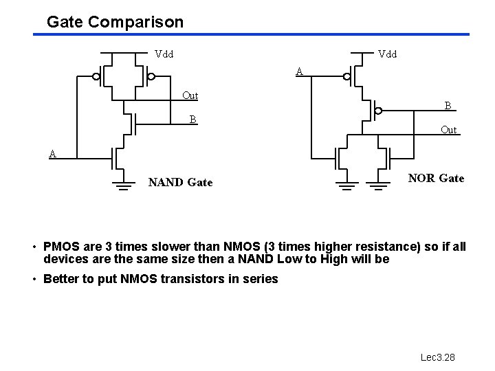
Gate Comparison Vdd A Out B B Out A NAND Gate NOR Gate • PMOS are 3 times slower than NMOS (3 times higher resistance) so if all devices are the same size then a NAND Low to High will be • Better to put NMOS transistors in series Lec 3. 28

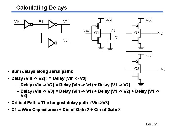
Calculating Delays Vin V 1 Vdd V 2 Vin G 1 V 3 Vdd V 1 G 2 V 2 C 1 Vdd • Sum delays along serial paths G 3 V 3 • Delay (Vin -> V 2) ! = Delay (Vin -> V 3) – Delay (Vin -> V 2) = Delay (Vin -> V 1) + Delay (V 1 -> V 2) – Delay (Vin -> V 3) = Delay (Vin -> V 1) + Delay (V 1 -> V 2) + Delay (V 1 -> V 3) • Critical Path = The longest delay path (Vin->V 3) • C 1 = Wire Capacitance + Cin of Gate 2 + Cin of Gate 3 Lec 3. 29

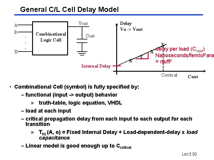
General C/L Cell Delay Model A B X Vout. . . Combinational Logic Cell Delay Va -> Vout Cout X X Internal Delay X delay per load (Cload) X Nanoseconds/femto. Fara = ns/f. F Ccritical Cout • Combinational Cell (symbol) is fully specified by: – functional (input -> output) behavior » truth-table, logic equation, VHDL – load at each input – critical propagation delay from each input to each output for each transition » THL(A, o) = Fixed Internal Delay + Load-dependent-delay x load capacitance – Linear model is good enough up to Ccritical Lec 3. 30

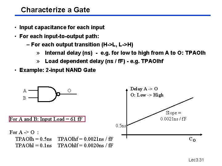
Characterize a Gate • Input capacitance for each input • For each input-to-output path: – For each output transition (H->L, L->H) » Internal delay (ns) - e. g. for low to high from A to O: TPAOlh » Load dependent delay (ns / f. F) - e. g. TPAOlhf • Example: 2 -input NAND Gate A B Delay A -> O O: Low -> High O Slope = 0. 0021 ns / f. F For A and B: Input Load = 61 f. F 0. 5 ns For A -> O : TPAOlh = 0. 5 ns TPAOhl = 0. 1 ns TPAOlhf = 0. 0021 ns / f. F TPAOhlf = 0. 0020 ns / f. F CO Lec 3. 31

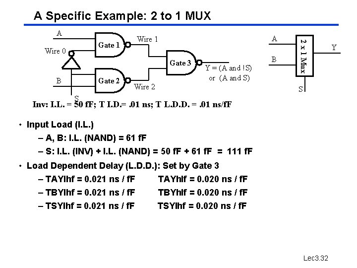
A Specific Example: 2 to 1 MUX A Gate 3 B Gate 2 Y = (A and !S) or (A and S) Wire 2 B 2 x 1 Mux Gate 1 Wire 0 A Wire 1 S S Inv: I. L. = 50 f. F; T I. D. =. 01 ns; T L. D. D. =. 01 ns/f. F • Input Load (I. L. ) – A, B: I. L. (NAND) = 61 f. F – S: I. L. (INV) + I. L. (NAND) = 50 f. F + 61 f. F = 111 f. F • Load Dependent Delay (L. D. D. ): Set by Gate 3 – TAYlhf = 0. 021 ns / f. F TAYhlf = 0. 020 ns / f. F – TBYlhf = 0. 021 ns / f. F TBYhlf = 0. 020 ns / f. F – TSYlhf = 0. 021 ns / f. F TSYlhf = 0. 020 ns / f. F Lec 3. 32 Y

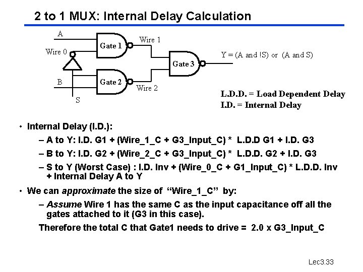
2 to 1 MUX: Internal Delay Calculation A Gate 1 Wire 0 Wire 1 Y = (A and !S) or (A and S) Gate 3 B Gate 2 S Wire 2 L. D. D. = Load Dependent Delay I. D. = Internal Delay • Internal Delay (I. D. ): – A to Y: I. D. G 1 + (Wire_1_C + G 3_Input_C) * L. D. D G 1 + I. D. G 3 – B to Y: I. D. G 2 + (Wire_2_C + G 3_Input_C) * L. D. D. G 2 + I. D. G 3 – S to Y (Worst Case) : I. D. Inv + (Wire_0_C + G 1_Input_C) * L. D. D. Inv + Internal Delay A to Y • We can approximate the size of “Wire_1_C” by: – Assume Wire 1 has the same C as the input capacitance off all the gates attached to it (G 3 in this case). Therefore the total C that Gate 1 needs to drive = 2. 0 x G 3_Input_C Lec 3. 33

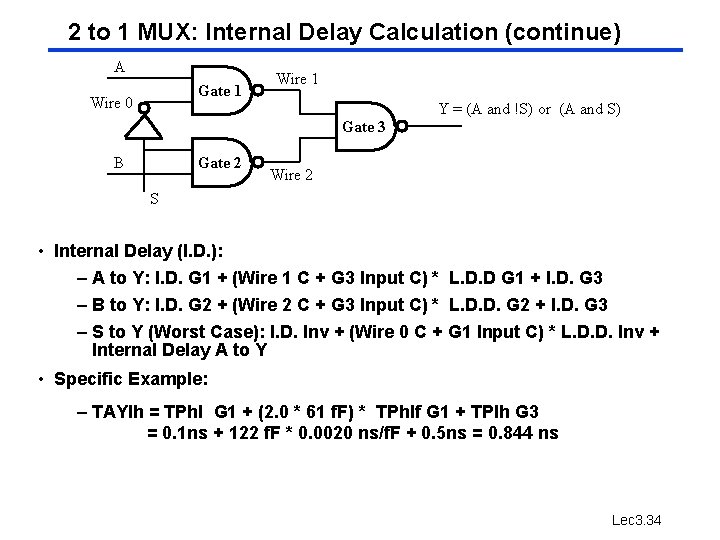
2 to 1 MUX: Internal Delay Calculation (continue) A Gate 1 Wire 0 Wire 1 Y = (A and !S) or (A and S) Gate 3 B Gate 2 Wire 2 S • Internal Delay (I. D. ): – A to Y: I. D. G 1 + (Wire 1 C + G 3 Input C) * L. D. D G 1 + I. D. G 3 – B to Y: I. D. G 2 + (Wire 2 C + G 3 Input C) * L. D. D. G 2 + I. D. G 3 – S to Y (Worst Case): I. D. Inv + (Wire 0 C + G 1 Input C) * L. D. D. Inv + Internal Delay A to Y • Specific Example: – TAYlh = TPhl G 1 + (2. 0 * 61 f. F) * TPhlf G 1 + TPlh G 3 = 0. 1 ns + 122 f. F * 0. 0020 ns/f. F + 0. 5 ns = 0. 844 ns Lec 3. 34

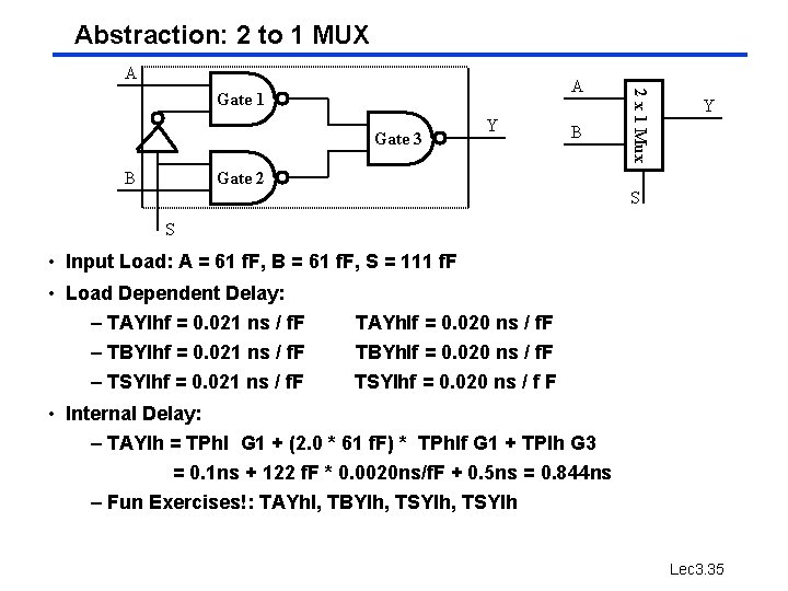
Abstraction: 2 to 1 MUX A Gate 3 B Y B 2 x 1 Mux A Gate 1 Y Gate 2 S S • Input Load: A = 61 f. F, B = 61 f. F, S = 111 f. F • Load Dependent Delay: – TAYlhf = 0. 021 ns / f. F – TBYlhf = 0. 021 ns / f. F – TSYlhf = 0. 021 ns / f. F TAYhlf = 0. 020 ns / f. F TBYhlf = 0. 020 ns / f. F TSYlhf = 0. 020 ns / f F • Internal Delay: – TAYlh = TPhl G 1 + (2. 0 * 61 f. F) * TPhlf G 1 + TPlh G 3 = 0. 1 ns + 122 f. F * 0. 0020 ns/f. F + 0. 5 ns = 0. 844 ns – Fun Exercises!: TAYhl, TBYlh, TSYlh Lec 3. 35

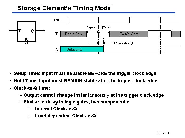
Storage Element’s Timing Model Clk D Q Setup D Don’t Care Hold Don’t Care Clock-to-Q Q Unknown • Setup Time: Input must be stable BEFORE the trigger clock edge • Hold Time: Input must REMAIN stable after the trigger clock edge • Clock-to-Q time: – Output cannot change instantaneously at the trigger clock edge – Similar to delay in logic gates, two components: » Internal Clock-to-Q » Load dependent Clock-to-Q Lec 3. 36

CS 152 Building blocks (maybe more…. ) • Logic elements – NAND 2, NAND 3, NAND 4 – NOR 2, NOR 3, NOR 4 – INV 1 x (normal inverter) – INV 4 x (inverter with large output drive) – XOR 2 – XNOR 2 – PWR: Source of 1’s – GND: Source of 0’s – fast MUXes • Storage Element – D flip flop - negative edge triggered Lec 3. 37

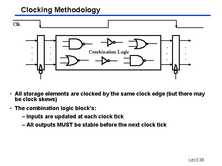
Clocking Methodology Clk . . . Combination Logic . . . • All storage elements are clocked by the same clock edge (but there may be clock skews) • The combination logic block’s: – Inputs are updated at each clock tick – All outputs MUST be stable before the next clock tick Lec 3. 38

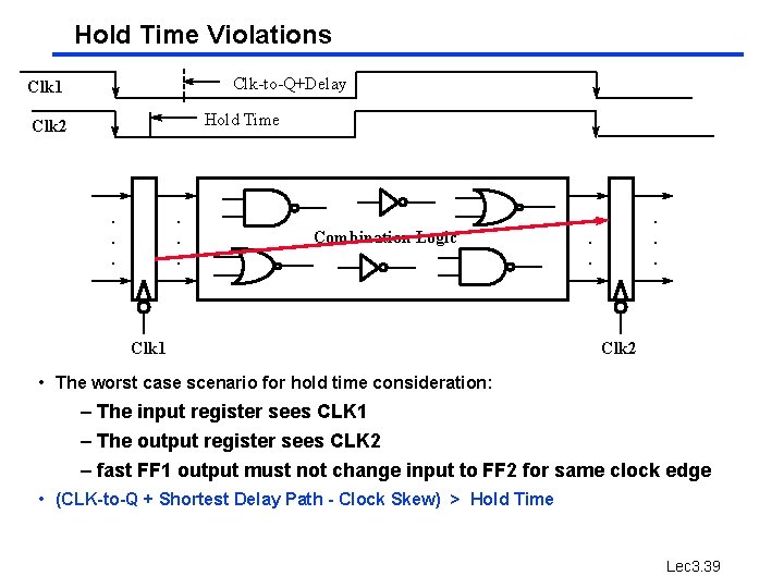
Hold Time Violations Clk-to-Q+Delay Clk 1 Hold Time Clk 2 . . . Combination Logic Clk 1 . . . Clk 2 • The worst case scenario for hold time consideration: – The input register sees CLK 1 – The output register sees CLK 2 – fast FF 1 output must not change input to FF 2 for same clock edge • (CLK-to-Q + Shortest Delay Path - Clock Skew) > Hold Time Lec 3. 39

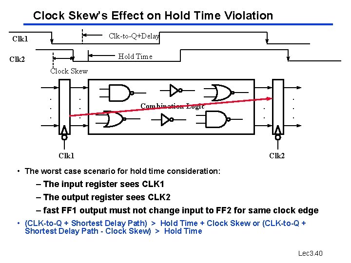
Clock Skew’s Effect on Hold Time Violation Clk-to-Q+Delay Clk 1 Hold Time Clk 2 Clock Skew. . . Combination Logic Clk 1 . . . Clk 2 • The worst case scenario for hold time consideration: – The input register sees CLK 1 – The output register sees CLK 2 – fast FF 1 output must not change input to FF 2 for same clock edge • (CLK-to-Q + Shortest Delay Path) > Hold Time + Clock Skew or (CLK-to-Q + Shortest Delay Path - Clock Skew) > Hold Time Lec 3. 40

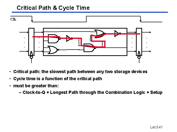
Critical Path & Cycle Time Clk . . . • Critical path: the slowest path between any two storage devices • Cycle time is a function of the critical path • must be greater than: – Clock-to-Q + Longest Path through the Combination Logic + Setup Lec 3. 41

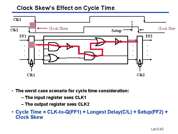
Clock Skew’s Effect on Cycle Time Clk 1 Clock Skew Clk 2 Clock Skw Setup FF 1 FF 2 . . . Clk 1 . . . Clk 2 • The worst case scenario for cycle time consideration: – The input register sees CLK 1 – The output register sees CLK 2 • Cycle Time = CLK-to-Q(FF 1) + Longest Delay(C/L) + Setup(FF 2) + Clock Skew Lec 3. 42

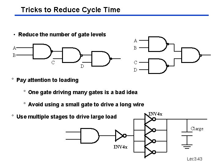
Tricks to Reduce Cycle Time • Reduce the number of gate levels A B C C D D ° Pay attention to loading ° One gate driving many gates is a bad idea ° Avoid using a small gate to drive a long wire ° Use multiple stages to drive large load INV 4 x Clarge INV 4 x Lec 3. 43

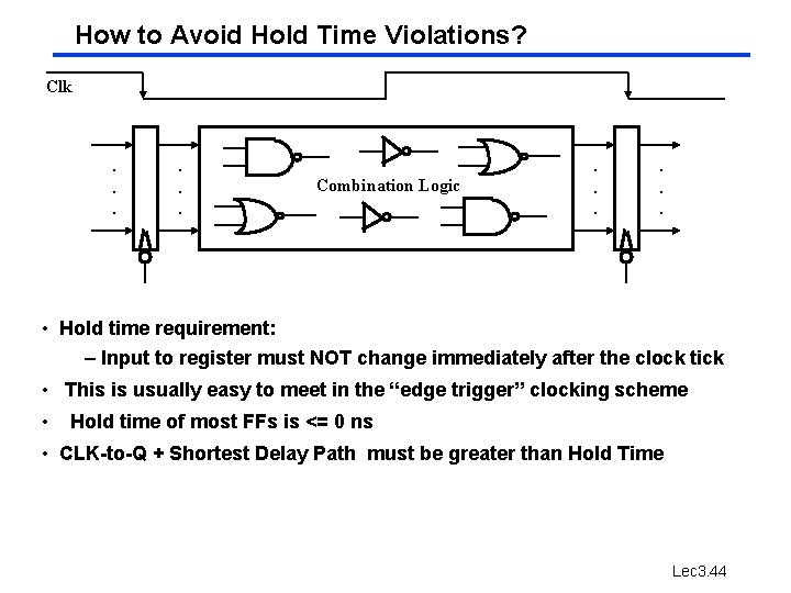
How to Avoid Hold Time Violations? Clk . . . Combination Logic . . . • Hold time requirement: – Input to register must NOT change immediately after the clock tick • This is usually easy to meet in the “edge trigger” clocking scheme • Hold time of most FFs is <= 0 ns • CLK-to-Q + Shortest Delay Path must be greater than Hold Time Lec 3. 44

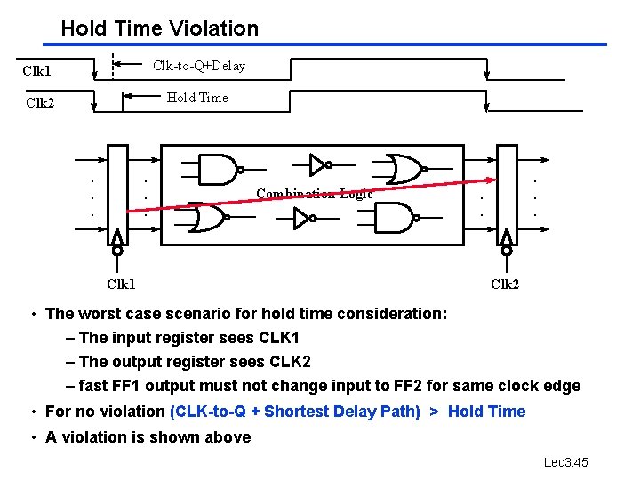
Hold Time Violation Clk 1 Clk-to-Q+Delay Clk 2 Hold Time . . . Clk 1 Combination Logic . . . Clk 2 • The worst case scenario for hold time consideration: – The input register sees CLK 1 – The output register sees CLK 2 – fast FF 1 output must not change input to FF 2 for same clock edge • For no violation (CLK-to-Q + Shortest Delay Path) > Hold Time • A violation is shown above Lec 3. 45

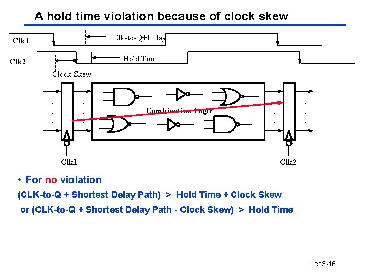
A hold time violation because of clock skew Clk-to-Q+Delay Clk 1 Hold Time Clk 2 Clock Skew. . . Clk 1 Combination Logic . . . Clk 2 • For no violation (CLK-to-Q + Shortest Delay Path) > Hold Time + Clock Skew or (CLK-to-Q + Shortest Delay Path - Clock Skew) > Hold Time Lec 3. 46

Summary • Total execution time is the most reliable measure of performance • Amdall’s law: Law of Diminishing Returns • Performance and Technology Trends – Keep the design simple (KISS rule) to take advantage of the latest technology – CMOS inverter and CMOS logic gates • Delay Modeling and Gate Characterization – Delay = Internal Delay + (Load Dependent Delay x Output Load) • Clocking Methodology and Timing Considerations – Simplest clocking methodology » All storage elements use the SAME clock edge – Cycle Time CLK-to-Q + Longest Delay Path + Setup + Clock Skew – (CLK-to-Q + Shortest Delay Path - Clock Skew) > Hold Time Lec 3. 47

To Get More Information • EECS 141 - Digital Integrated Circuit Design - 105 no longer a prerequisite - only EECS 40 required! • Book: Digital Integrated Circuits - A design perspective - by Jan Rabaey • Web page (slides from book) – http: //bwrc. eecs. berkeley. edu/icdesign/instructors. html Lec 3. 48