Conditional Convergence and LongRun Economic Growth Mr Vaughan

Conditional Convergence and Long-Run Economic Growth Mr. Vaughan Income and Employment Theory (402) Updated: 2/23/09 1

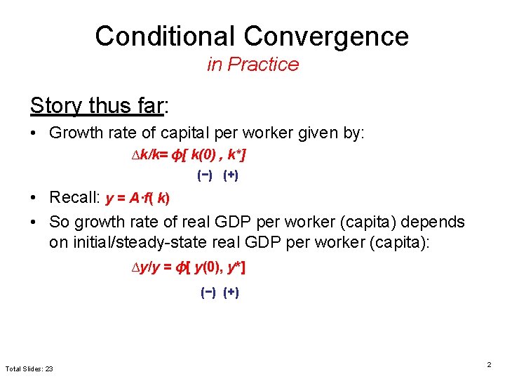
Conditional Convergence in Practice Story thus far: • Growth rate of capital per worker given by: ∆k/k= ϕ[ k(0) , k*] (−) (+) • Recall: y = A·f( k) • So growth rate of real GDP per worker (capita) depends on initial/steady-state real GDP per worker (capita): ∆y/y = ϕ[ y(0), y*] (−) (+) Total Slides: 23 2

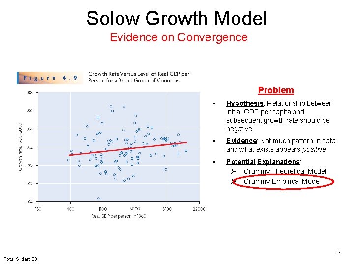
Solow Growth Model Evidence on Convergence Problem • Hypothesis: Relationship between initial GDP per capita and subsequent growth rate should be negative. • Evidence: Not much pattern in data, and what exists appears positive. • Potential Explanations: Ø Crummy Theoretical Model Ø Crummy Empirical Model 3 Total Slides: 23

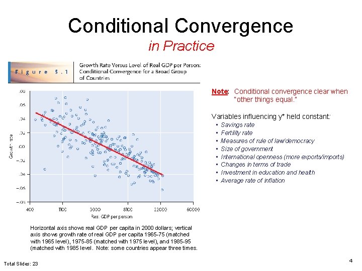
Conditional Convergence in Practice Note: Conditional convergence clear when “other things equal. ” Variables influencing y* held constant: • • Savings rate Fertility rate Measures of rule of law/democracy Size of government International openness (more exports/imports) Changes in terms of trade Investment in education and health Average rate of inflation Horizontal axis shows real GDP per capita in 2000 dollars; vertical axis shows growth rate of real GDP per capita 1965 -75 (matched with 1965 level), 1975 -85 (matched with 1975 level), and 1985 -95 (matched with 1985 level. Note: some countries appear three times. Total Slides: 23 4

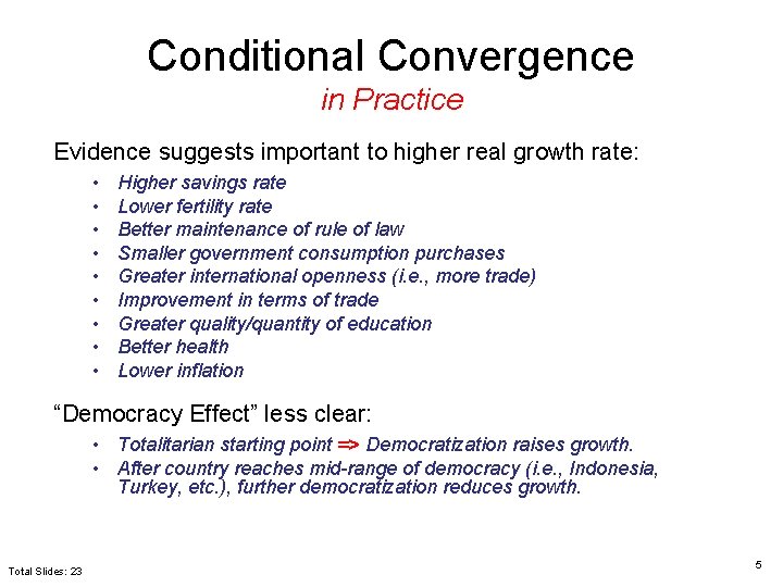
Conditional Convergence in Practice Evidence suggests important to higher real growth rate: • • • Higher savings rate Lower fertility rate Better maintenance of rule of law Smaller government consumption purchases Greater international openness (i. e. , more trade) Improvement in terms of trade Greater quality/quantity of education Better health Lower inflation “Democracy Effect” less clear: • Totalitarian starting point => Democratization raises growth. • After country reaches mid-range of democracy (i. e. , Indonesia, Turkey, etc. ), further democratization reduces growth. Total Slides: 23 5

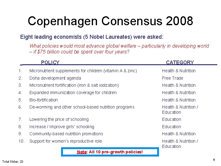
Copenhagen Consensus 2008 Eight leading economists (5 Nobel Laureates) were asked: What policies would most advance global welfare – particularly in developing world – if $75 billion could be spent over four years? POLICY CATEGORY 1. Micronutrient supplements for children (vitamin A & zinc) Health & Nutrition 2. Doha development agenda Free Trade 3. Micronutrient fortification (iron & salt iodization) Health & Nutrition 4. Expanded immunization coverage for children Health & Nutrition 5. Bio-fortification Health & Nutrition 6. De-worming and other school-based nutrition programs Health & Nutrition / Education 7. Lowering the price of schooling Education 8. Increase / Improve girls’ schooling Education 9. Community-based nutrition promotions Health & Nutrition 10. Support for women’s reproductive role Health & Nutrition / Education Note: All 10 pro-growth policies! Total Slides: 23 6

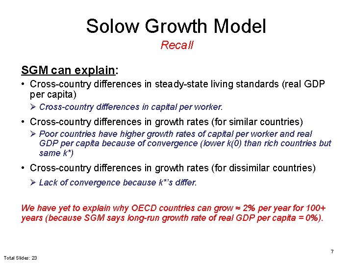
Solow Growth Model Recall SGM can explain: • Cross-country differences in steady-state living standards (real GDP per capita) Ø Cross-country differences in capital per worker. • Cross-country differences in growth rates (for similar countries) Ø Poor countries have higher growth rates of capital per worker and real GDP per capita because of convergence (lower k(0) than rich countries but same k*) • Cross-country differences in growth rates (for dissimilar countries) Ø Lack of convergence because k*’s differ. We have yet to explain why OECD countries can grow ≈ 2% per year for 100+ years (because SGM says long-run growth rate of real GDP per capita = 0%). 7 Total Slides: 23

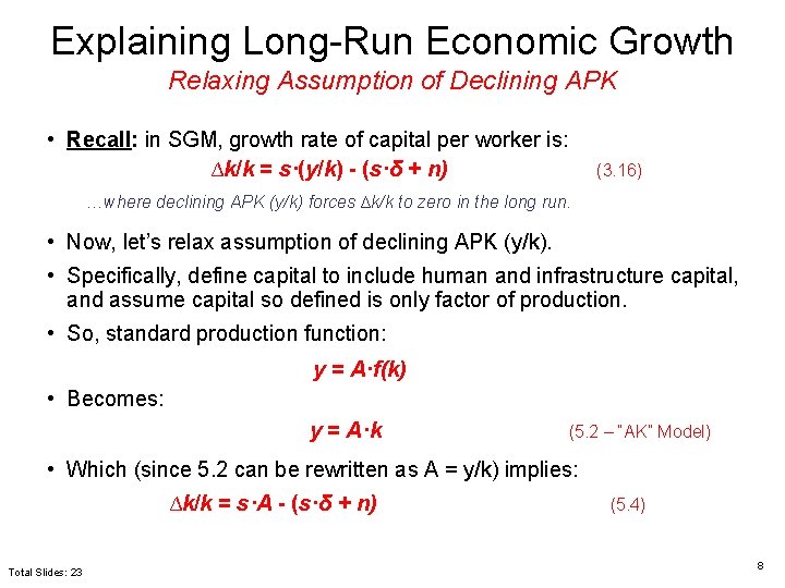
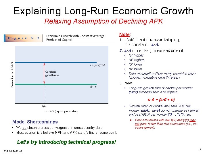
Explaining Long-Run Economic Growth Relaxing Assumption of Declining APK • Recall: in SGM, growth rate of capital per worker is: ∆k/k = s·(y/k) - (s·δ + n) (3. 16) …where declining APK (y/k) forces ∆k/k to zero in the long run. • Now, let’s relax assumption of declining APK (y/k). • Specifically, define capital to include human and infrastructure capital, and assume capital so defined is only factor of production. • So, standard production function: y = A·f(k) • Becomes: y = A·k (5. 2 – “AK” Model) • Which (since 5. 2 can be rewritten as A = y/k) implies: ∆k/k = s·A - (s·δ + n) Total Slides: 23 (5. 4) 8

Explaining Long-Run Economic Growth Relaxing Assumption of Declining APK Note: 1. s(y/k) is not downward-sloping; it is constant = s·A. 2. s·A more likely to exceed sδ+n if: • • • “s” higher “A” higher “δ” lower “n” lower Safe assumption (how many countries have long-term negative growth rates)? 3. Now: • Long-run growth rate of capital per worker (∆k/k) exceeds zero and equals: s·A − (s·δ + n) • Growth rates of capital and real GDP per worker (∆k/k, ∆y/y) do not change as capital and real GDP per worker (“k” , “y”) rise. Model Shortcomings • We do observe cross-convergence in cross-country data. • Most economists believe MPK and APK start falling at some point. Ø Poor economies with low k(0) and y(0) may not grow faster than rich economies (i. e. , no convergence). Let’s try introducing technical progress! Total Slides: 23 9

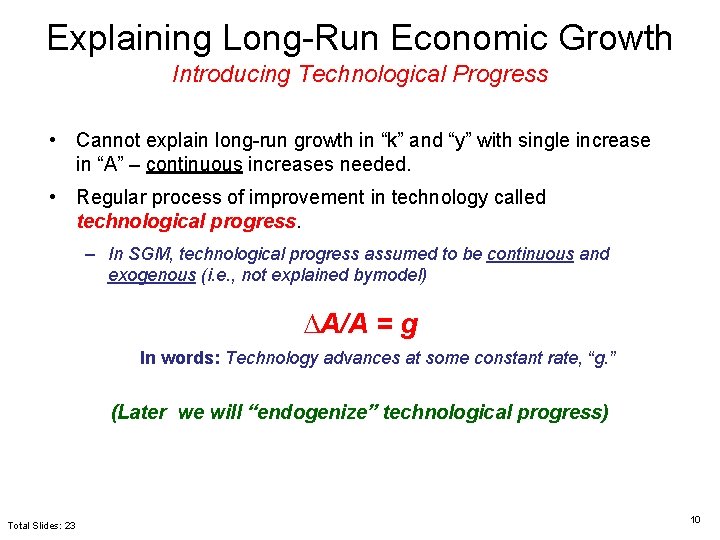
Explaining Long-Run Economic Growth Introducing Technological Progress • Cannot explain long-run growth in “k” and “y” with single increase in “A” – continuous increases needed. • Regular process of improvement in technology called technological progress. – In SGM, technological progress assumed to be continuous and exogenous (i. e. , not explained bymodel) ∆A/A = g In words: Technology advances at some constant rate, “g. ” (Later we will “endogenize” technological progress) Total Slides: 23 10

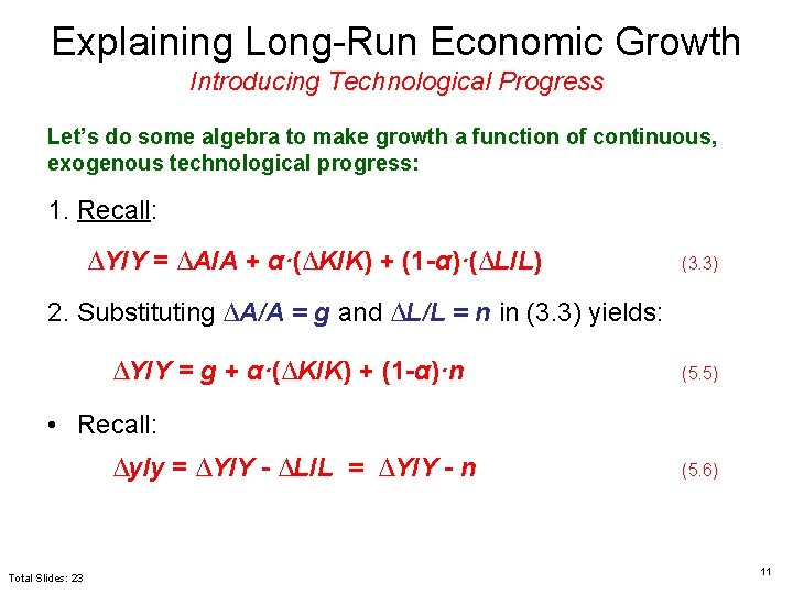
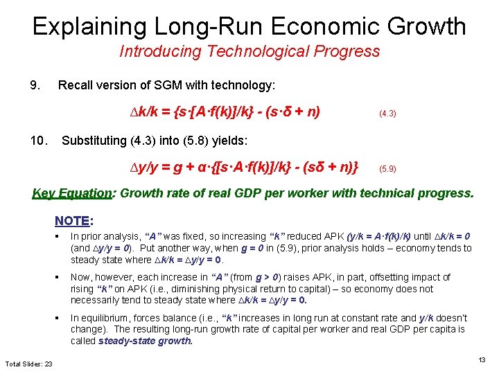
Explaining Long-Run Economic Growth Introducing Technological Progress Let’s do some algebra to make growth a function of continuous, exogenous technological progress: 1. Recall: ∆Y/Y = ∆A/A + α·(∆K/K) + (1 -α)·(∆L/L) (3. 3) 2. Substituting ∆A/A = g and ∆L/L = n in (3. 3) yields: ∆Y/Y = g + α·(∆K/K) + (1 -α)·n (5. 5) • Recall: ∆y/y = ∆Y/Y - ∆L/L = ∆Y/Y - n Total Slides: 23 (5. 6) 11

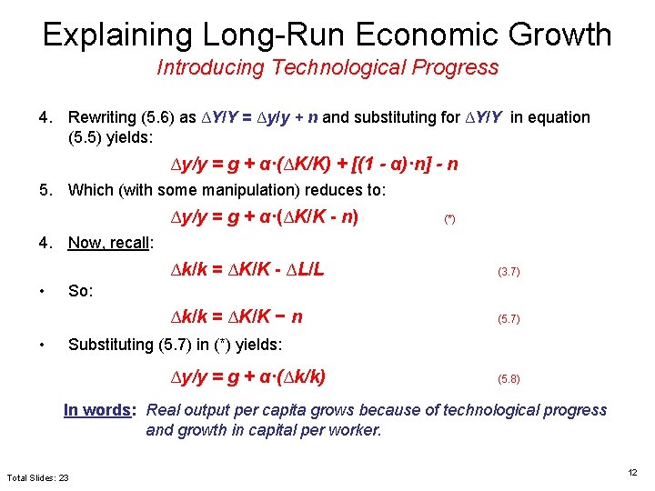
Explaining Long-Run Economic Growth Introducing Technological Progress 4. Rewriting (5. 6) as ∆Y/Y = ∆y/y + n and substituting for ∆Y/Y in equation (5. 5) yields: ∆y/y = g + α·(∆K/K) + [(1 - α)·n] - n 5. Which (with some manipulation) reduces to: ∆y/y = g + α·(∆K/K - n) (*) 4. Now, recall: • • ∆k/k = ∆K/K - ∆L/L (3. 7) ∆k/k = ∆K/K − n (5. 7) So: Substituting (5. 7) in (*) yields: ∆y/y = g + α·(∆k/k) (5. 8) In words: Real output per capita grows because of technological progress and growth in capital per worker. Total Slides: 23 12

Explaining Long-Run Economic Growth Introducing Technological Progress 9. Recall version of SGM with technology: ∆k/k = {s·[A·f(k)]/k} - (s·δ + n) 10. (4. 3) Substituting (4. 3) into (5. 8) yields: ∆y/y = g + α·{[s·A·f(k)]/k} - (sδ + n)} (5. 9) Key Equation: Growth rate of real GDP per worker with technical progress. NOTE: Total Slides: 23 § In prior analysis, “A” was fixed, so increasing “k” reduced APK (y/k = A·f(k)/k) until ∆k/k = 0 (and ∆y/y = 0). Put another way, when g = 0 in (5. 9), prior analysis holds – economy tends to steady state where ∆k/k = ∆y/y = 0. § Now, however, each increase in “A” (from g > 0) raises APK, in part, offsetting impact of rising “k” on APK (i. e. , diminishing physical return to capital) – so economy does not necessarily tend to steady state where ∆k/k = ∆y/y = 0. § In equilibrium, forces balance (i. e. , “k” increases in long run at constant rate and y/k doesn’t change). The resulting long-run growth rate of capital per worker and real GDP per capita is called steady-state growth. 13

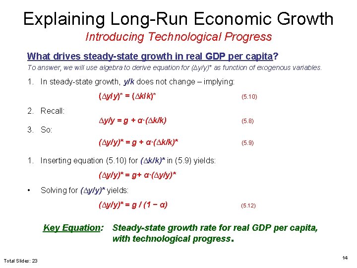
Explaining Long-Run Economic Growth Introducing Technological Progress What drives steady-state growth in real GDP per capita? To answer, we will use algebra to derive equation for (∆y/y)* as function of exogenous variables. 1. In steady-state growth, y/k does not change – implying: (∆y/y)* = (∆k/k)* (5. 10) ∆y/y = g + α·(∆k/k) (5. 8) (∆y/y)* = g + α·(∆k/k)* (5. 9) 2. Recall: 3. So: 1. Inserting equation (5. 10) for (∆k/k)* in (5. 9) yields: (∆y/y)* = g+ α·(∆y/y)* • Solving for (∆y/y)* yields: (∆y/y)* = g / (1 − α) Key Equation: Total Slides: 23 (5. 12) Steady-state growth rate for real GDP per capita, with technological progress. 14

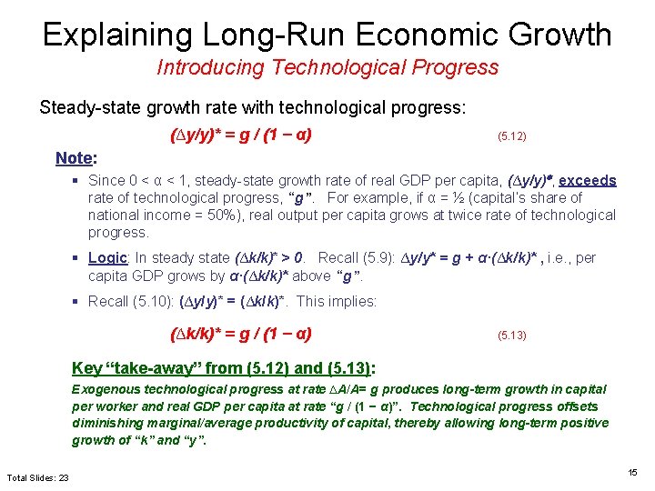
Explaining Long-Run Economic Growth Introducing Technological Progress Steady-state growth rate with technological progress: (∆y/y)* = g / (1 − α) (5. 12) Note: § Since 0 < α < 1, steady-state growth rate of real GDP per capita, (∆y/y)∗, exceeds rate of technological progress, “g”. For example, if α = ½ (capital’s share of national income = 50%), real output per capita grows at twice rate of technological progress. § Logic: In steady state (∆k/k)* > 0. Recall (5. 9): ∆y/y* = g + α·(∆k/k)* , i. e. , per capita GDP grows by α·(∆k/k)* above “g”. § Recall (5. 10): (∆y/y)* = (∆k/k)*. This implies: (∆k/k)* = g / (1 − α) (5. 13) Key “take-away” from (5. 12) and (5. 13): Exogenous technological progress at rate ∆A/A= g produces long-term growth in capital per worker and real GDP per capita at rate “g / (1 − α)”. Technological progress offsets diminishing marginal/average productivity of capital, thereby allowing long-term positive growth of “k” and “y”. Total Slides: 23 15

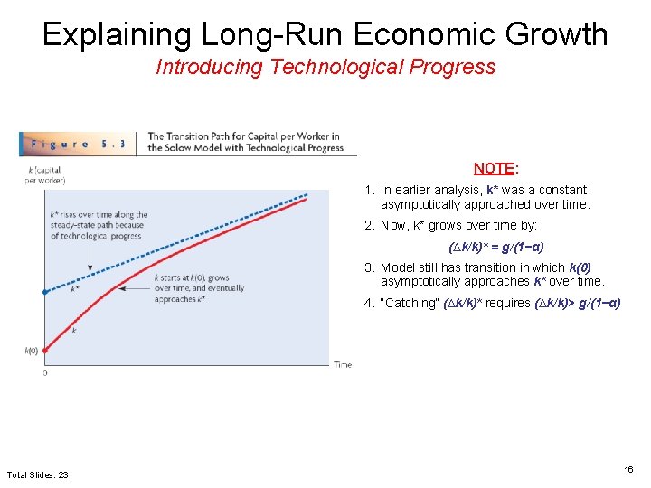
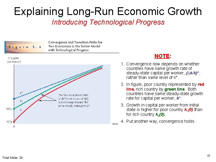
Explaining Long-Run Economic Growth Introducing Technological Progress NOTE: 1. In earlier analysis, k* was a constant asymptotically approached over time. 2. Now, k* grows over time by: (∆k/k)* = g/(1−α) 3. Model still has transition in which k(0) asymptotically approaches k* over time. 4. “Catching” (∆k/k)* requires (∆k/k)> g/(1−α) Total Slides: 23 16

Explaining Long-Run Economic Growth Introducing Technological Progress NOTE: 1. Convergence now depends on whether countries have same growth rate of steady-state capital per worker, (∆k/k)*, rather than same level of k*. 2. In figure, poor country represented by red line, rich country by green line. Both countries have same steady-state growth rate for capital per worker, k*. 3. Growth in capital per worker from initial state is higher for poor country k 1(0) than for rich country k 2(0). 4. Put another way, convergence holds. Total Slides: 23 17

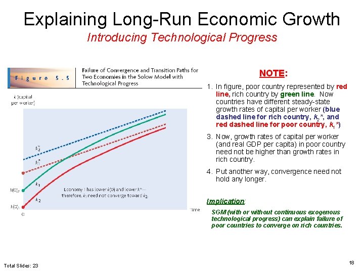
Explaining Long-Run Economic Growth Introducing Technological Progress NOTE: 1. In figure, poor country represented by red line, rich country by green line. Now countries have different steady-state growth rates of capital per worker (blue dashed line for rich country, k 2*, and red dashed line for poor country, k 1*) 3. Now, growth rates of capital per worker (and real GDP per capita) in poor country need not be higher than growth rates in rich country. 4. Put another way, convergence need not hold any longer. Implication: SGM (with or without continuous exogenous technological progress) can explain failure of poor countries to converge on rich countries. Total Slides: 23 18

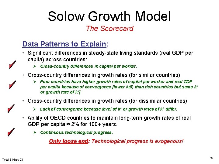
Solow Growth Model The Scorecard Data Patterns to Explain: • Significant differences in steady-state living standards (real GDP per capita) across countries: Ø Cross-country differences in capital per worker. • Cross-country differences in growth rates (for similar countries) Ø Poor countries have higher growth rates of capital per worker and real GDP per capita because of convergence [lower k(0) than rich countries but same k* or growth rate of k*] • Cross-country differences in growth rates (for dissimilar countries) Ø Lack of convergence because level of k* or growth rates of k* differ. • Ability of OECD countries to maintain long-term growth rates of real GDP per capita ≈ 2% for 100+ years. Ø Continuous technological progress. Only loose end: Technological progress is exogenous! Total Slides: 23 19

Endogenous Growth Theory (founded by Paul Romer) § Called “endogenous” because models: a) Extend SGM to explain rate of technological progress, and… b) Technological progress produces positive long-run growth of capital per worker/real GDP per capita [as in SGM]. § Most endogenous growth models driven by investments in research and development (R&D): a) Technological progress represented by increases in “A” (in SGM framework). b) More R&D implies more technological progress (discovery of new/better products or superior methods of production), other things equal. c) Marginal returns on R&D-driven technological progress do not decline (i. e. , good ideas unlimited) => produces constant growth rate (g) for “A” (like SGM). d) Other things equal, factors raising private-sector return to R&D lead to more R&D: Ø Lower costs of R&D (e. g. , government subsidies of research) Ø Higher potential sales revenues/lower production costs from R&D investment (e. g. , larger market for selling fruits of R&D => explain links between free trade and growth). Ø More secure (and long-lasting) intellectual property rights over use of inventions from R&D. Total Slides: 23 20

Endogenous Growth Theory (founded by Paul Romer) Empirical Evidence: § Countries spending most on R&D, other things equal, have higher growth rates of real GDP per capita. § Advanced countries spend most on R&D (explains high long-term OECD growth rates). § Poor countries can raise level of technology by imitating/adapting innovations from other countries (Diffusion of Technology) Ø Another potential source of convergence (high growth rate initially, but opportunities for additional profitable imitation decline). Ø Rate of technological innovation to developing country is high, other things equal, when that country : – Trades extensively with rich countries. – Has high education levels. Helps explain high growth rates of East Asian countries since 1960! – Has well-functioning legal/political systems. Total Slides: 23 21

Thought Questions • Based on what you have learned, what explains poor growth record in Sub-Saharan Africa? • What policies would you recommend to boost growth/alleviate poverty and why? *** • What policies would you recommend to President Obama to boost long-term U. S. growth? Total Slides: 23 22

Questions over Conditional Convergence and Long-Run Economic Growth Mr. Vaughan Income and Employment Theory (402) Total Slides: 23 23