COMPUTER GRAPHICS 2 D TRANSFORMATIONS 2 D Transformations

COMPUTER GRAPHICS 2 D TRANSFORMATIONS

2 D Transformations “Transformations are the operations applied to geometrical description of an object to change its position, orientation, or size are called geometric transformations”.

Why Transformations ? “Transformations are needed to manipulate the initially created object and to display the modified object without having to redraw it. ”

• Translation • Rotation

• Scaling • Uniform Scaling • Un-uniform Scaling

• Reflection • Shear

Translation • A translation moves all points in an object along the same straight-line path to new positions. • The path is represented by a vector, called the translation or shift vector. • We can write the components: p'x = px + tx p'y = py + ty • or in matrix form: P' = P + T tx x' x y' = y + ty P'(8, 6) ty=4 P(2, 2) tx= 6

Rotation • A rotation repositions all points in an object along a circular path in the plane centered at the pivot point. • First, we’ll assume the pivot is at the origin. P P

Rotation • Review Trigonometry => cos = x/r , sin = y/r • x = r. cos , y = r. sin => cos ( + ) = x’/r • x’ = r. cos ( + ) • x’ = r. cos -r. sin • x’ = x. cos – y. sin =>sin ( + ) = y’/r y’ = r. sin ( + ) • y’ = r. cos sin + r. sin cos • y’ = x. sin + y. cos P’(x’, y’) r y’ x’ P(x, y) r y x Identity of Trigonometry

Rotation • We can write the components: p'x = px cos – py sin p'y = px sin + py cos P’(x’, y’) • or in matrix form: P' = R • P • can be clockwise (-ve) or counterclockwise (+ve as our example). • Rotation matrix y’ x’ P(x, y) r x y

Scaling • Scaling changes the size of an object and involves two scale factors, Sx and Sy for the xand y- coordinates respectively. • Scales are about the origin. • We can write the components: p'x = sx • px p'y = sy • py or in matrix form: P' = S • P Scale matrix as: P’ P

Scaling • If the scale factors are in between 0 and 1: --- • the points will be moved closer to the origin • the object will be smaller. P(2, 5) P’ • Example : • P(2, 5), Sx = 0. 5, Sy = 0. 5

Scaling • If the scale factors are in between 0 and 1 the points will be moved closer to the origin the object will be smaller. • Example : • P(2, 5), Sx = 0. 5, Sy = 0. 5 • If the scale factors are larger than 1 the points will be moved away from the origin the object will be larger. • Example : • P(2, 5), Sx = 2, Sy = 2 P’ P(2, 5) P’

Scaling P’ • If the scale factors are the same, Sx = Sy uniform scaling • Only change in size (as previous example) • If Sx Sy differential scaling. • Change in size and shape • Example : square rectangle • P(1, 3), Sx = 2, Sy = 5 P(1, 2)

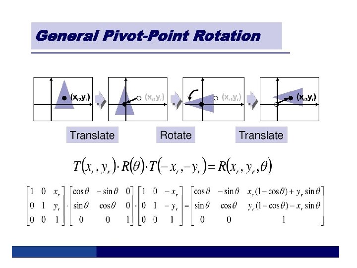
General pivot point rotation • Translate the object so that pivot-position is moved to the coordinate origin • Rotate the object about the coordinate origin • Translate the object so that the pivot point is returned to its original position (xr, yr) (a) (b) (c) (d) Original Position of Object and pivot point Translation of object so that pivot point (xr, yr) is at origin Rotation was about origin Translation of the object so that the pivot point is returned to position (xr, yr)

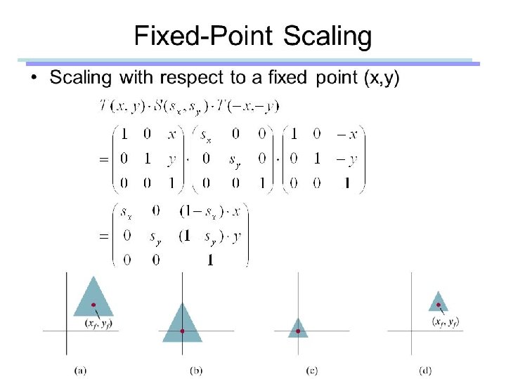
General fixed point scaling • Translate object so that the fixed point coincides with the coordinate origin • Scale the object with respect to the coordinate origin • Use the inverse translation of step 1 to return the object to its original position (xf, yf) (a) (b) Original Position of Object and Fixed point Translation of object so that fixed point (xf, yf)is at origin (c) (d) scaling was about origin Translation of the object so that the Fixed point is returned to position (xf, yf)

Composite Transformations (A) Translations If two successive translation vectors (tx 1, ty 1) and (tx 2, ty 2) are applied to a coordinate position P, the final transformed location P’ is calculated as: P’=T(tx 2, ty 2). {T(tx 1, ty 1). P} ={T(tx 2, ty 2). T(tx 1, ty 1)}. P Where P and P’ are represented as homogeneous-coordinate column vectors. We can verify this result by calculating the matrix product for the two associative groupings. Also, the composite transformation matrix for this sequence of transformations is: 1 0 tx 2 0 1 ty 2 0 1 0 . 0 1 ty 1 0 0 1 0 tx 1 1 = tx 1+tx 2 0 1 ty 1+ty 2 0 0 1 Or, T(tx 2, ty 2). T(tx 1, ty 1) = T(tx 1+tx 2, ty 1+ty 2) Which demonstrate that two successive translations are additive.

(B) Rotations Two successive rotations applied to point P produce the transformed position: P’= R(Ө 2). {R(Ө 1 ). P} = {R(Ө 2). R(Ө 1)}. P By multiplication the two rotation matrices, we can verify that two successive rotations are additive: R(Ө 2). R(Ө 1) = R (Ө 1+ Ө 2) So that the final rotated coordinates can be calculated with the composite rotation matrix as: P’ = R(Ө 1+ Ө 2). P

(C) Scaling Concatenating transformation matrices for two successive scaling operations produces the following composite scaling matrix: Sx 2 0 Or, Sx 1 0 0 0 Sy 2 0 0 0 1 . 0 0 Sy 1 0 0 0 1 = Sx 1. Sx 2 0 0 0 Sy 1. Sy 2 0 0 0 1 S(Sx 2, Sy 2 ). S(Sx 1, Sy 1) = S (Sx 1. Sx 2, Sy 1. Sy 2 ) The resulting matrix in this case indicates that successive scaling operations are multiplicative.

Other transformations • Reflection is a transformation that produces a mirror image of an object. It is obtained by rotating the object by 180 deg about the reflection axis 1 Original position 2 3 2’ 3’ Reflection about the line y=0, the X- axis , is accomplished with the transformation matrix 1 0 0 -1 0 0 1’ Reflected position 0 0 1

Reflection Original position Reflected position 2 2’ 1 3 1’ Reflection about the line x=0, the Y- axis , is accomplished with the transformation matrix 3’ -1 0 0 0 1

Reflection of an object relative to an axis perpendicular to the xy plane and passing through the coordinate origin Y-axis Reflected position 3’ -1 0 0 0 1 2’ 1’ Origin O 1 (0, 0) 2 3 Original position The above reflection matrix is X-axis the rotation matrix with angle=180 degree. This can be generalized to any reflection point in the xy plane. This reflection is the same as a 180 degree rotation in the xy plane using the reflection point as the pivot point.

Reflection of an object w. r. t the straight line y=x Y-axis Original position 3 2 0 1 0 0 1 1 1’ 3’ Reflected position 2’ Origin O (0, 0) X-axis

Reflection of an object w. r. t the Y-axis straight line y=-x 0 -1 0 0 0 X-axis 2 Origin O (0, 0) 3 1 Original position 1’ 2’ 3’ Reflected position Line Y = - X 0 1

Reflection of an arbitrary axis y=mx+b Original position 3 2 1

Original position 3 2 Translation so that it passes through origin Rotate so that it coincides with xaxis and reflect also about x-axis Original position 3 1 2 1 Original position 2 3 1 Translate back Rotate back Original position 3 2 1’ 2 1 1’ Reflected position 2’ 3’ 1 1’ 3’ 3’ 2’ Reflected position

Shear Transformations • Shear is a transformation that distorts the shape of an object such that the transformed shape appears as if the object were composed of internal layers that had been caused to slide over each other • Two common shearing transformations are those that shift coordinate x values and those that shift y values

Shears Original Data y Shear x Shear 1 0 0 shy 1 0 0 0 1 1 shx 0 0 1 0 0 0 1

An X- direction Shear For example, Shx=2 (2, 1) (0, 0) (1, 1) (1, 0) (0, 0) (1, 0) (3, 1)

An Y- direction Shear For example, Shy=2 Y Y (1, 3) (1, 2) (0, 1) (0, 0) (1, 1) (1, 0) (0, 1) X (0, 0) X

CONCLUSION To manipulate the initially created object and to display the modified object without having to redraw it, we use Transformations.

Textbook • Computer Graphics C Version – D. Hearn and M. P. Baker – 2 nd Edition – PRENTICE HALL

QUERY ?

THANK YOU ALL