Computational aspects of motor control and motor learning

Computational aspects of motor control and motor learning Michael I. Jordan* Mark J. Buller (mbuller) 21 February 2007 *In H. Heuer & S. Keele, (Eds. ), Handbook of Perception and Action: Motor Skills. New York: Academic Press, 1996.

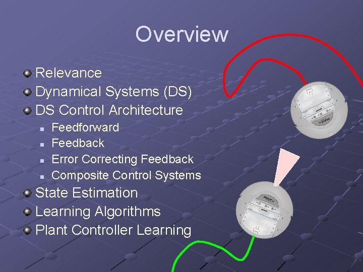
Overview Relevance Dynamical Systems (DS) DS Control Architecture n n Feedforward Feedback Error Correcting Feedback Composite Control Systems State Estimation Learning Algorithms Plant Controller Learning

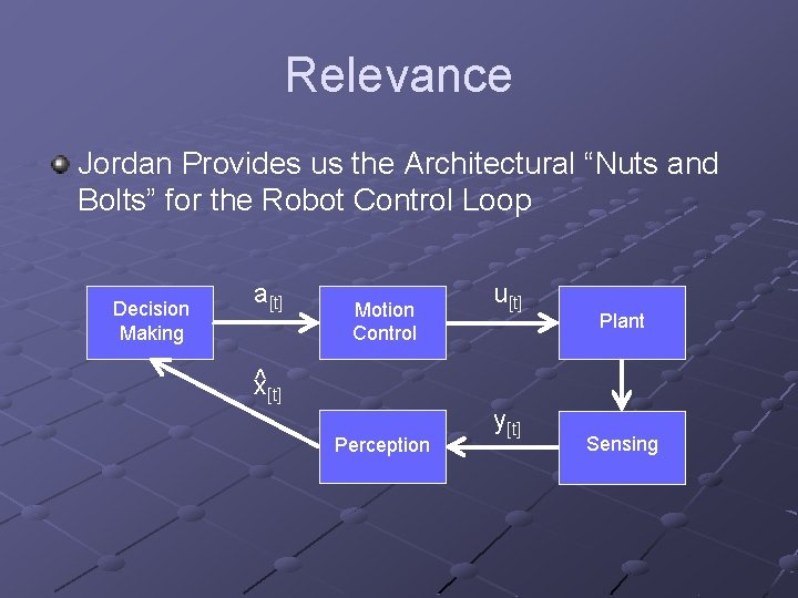
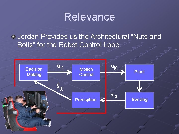
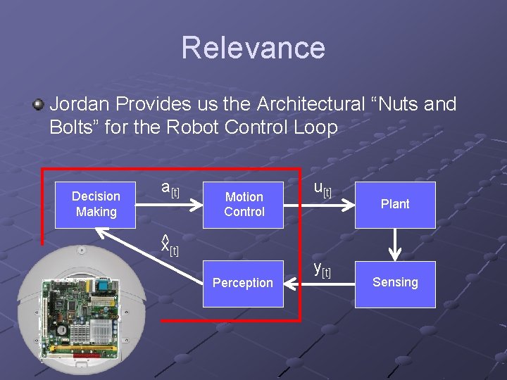
Relevance Jordan Provides us the Architectural “Nuts and Bolts” for the Robot Control Loop Decision Making a[t] Motion Control ^x[t] Perception u[t] y[t] Plant Sensing

Relevance Jordan Provides us the Architectural “Nuts and Bolts” for the Robot Control Loop Decision Making a[t] Motion Control ^x[t] Perception u[t] y[t] Plant Sensing

Relevance Jordan Provides us the Architectural “Nuts and Bolts” for the Robot Control Loop Decision Making a[t] Motion Control ^x[t] Perception u[t] y[t] Plant Sensing

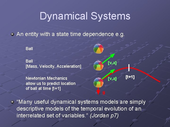
Dynamical Systems An entity with a state time dependence e. g. “Many useful dynamical systems models are simply descriptive models of the temporal evolution of an interrelated set of variables. ” (Jordan p 7)

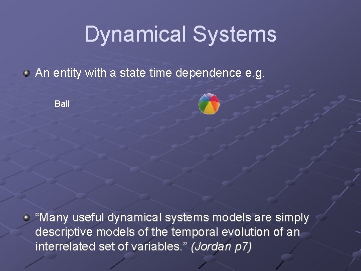
Dynamical Systems An entity with a state time dependence e. g. Ball “Many useful dynamical systems models are simply descriptive models of the temporal evolution of an interrelated set of variables. ” (Jordan p 7)

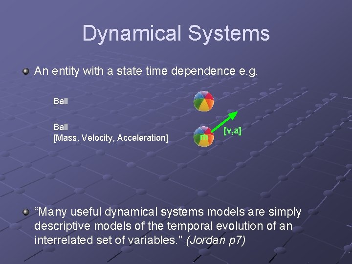
Dynamical Systems An entity with a state time dependence e. g. Ball [Mass, Velocity, Acceleration] m [v, a] “Many useful dynamical systems models are simply descriptive models of the temporal evolution of an interrelated set of variables. ” (Jordan p 7)

Dynamical Systems An entity with a state time dependence e. g. Ball [Mass, Velocity, Acceleration] Newtonian Mechanics allow us to predict location of ball at time [t+1] [v, a] m [t+1] g “Many useful dynamical systems models are simply descriptive models of the temporal evolution of an interrelated set of variables. ” (Jordan p 7)

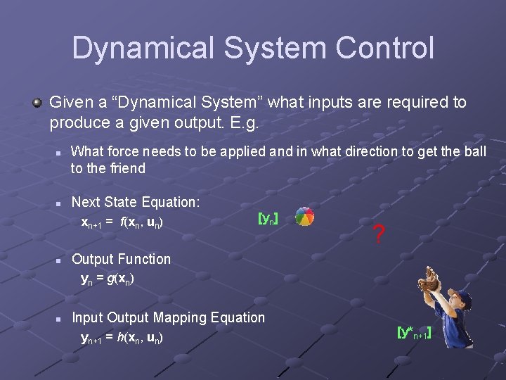
Dynamical System Control Given a “Dynamical System” what inputs are required to produce a given output. E. g. n n What force needs to be applied and in what direction to get the ball to the friend Next State Equation: xn+1 = f(xn, un) n [y n ] ? Output Function y n = g (x n ) n Input Output Mapping Equation yn+1 = h(xn, un) [y*n+1]

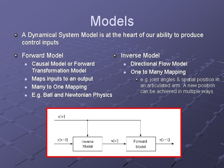
Models A Dynamical System Model is at the heart of our ability to produce control inputs Forward Model n n Causal Model or Forward Transformation Model Maps inputs to an output Many to One Mapping E. g. Ball and Newtonian Physics Inverse Model n n Directional Flow Model One to Many Mapping e. g. joint angles & spatial position In an articulated arm. A new position can be achieved in multiple ways

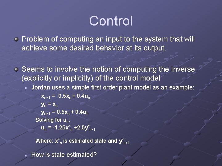
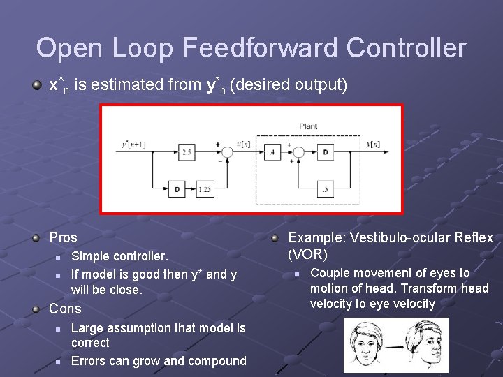
Control Problem of computing an input to the system that will achieve some desired behavior at its output. Seems to involve the notion of computing the inverse (explicitly or implicitly) of the control model n Jordan uses a simple first order plant model as an example: xn+1 = 0. 5 xn + 0. 4 un yn = xn yn+1 = 0. 5 xn + 0. 4 un Solving for un: un = -1. 25 x^n +2. 5 y*n+1 Where: x^n is estimated state and y*n+1 n How is state estimated?

Open Loop Feedforward Controller x^n is estimated from y*n (desired output) Pros n n Simple controller. If model is good then y* and y will be close. Cons n n Large assumption that model is correct Errors can grow and compound Example: Vestibulo-ocular Reflex (VOR) n Couple movement of eyes to motion of head. Transform head velocity to eye velocity

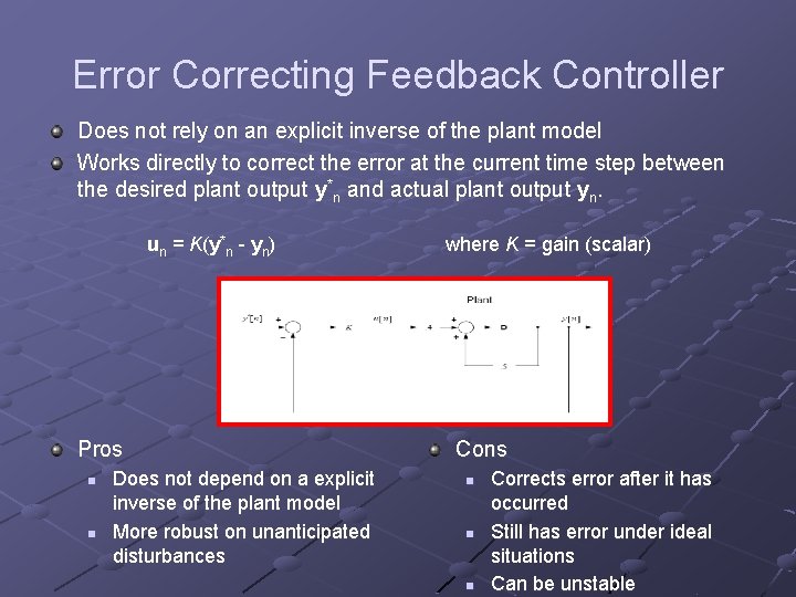
Error Correcting Feedback Controller Does not rely on an explicit inverse of the plant model Works directly to correct the error at the current time step between the desired plant output y*n and actual plant output yn. u n = K (y * n - y n ) Pros n n Does not depend on a explicit inverse of the plant model More robust on unanticipated disturbances where K = gain (scalar) Cons n n n Corrects error after it has occurred Still has error under ideal situations Can be unstable

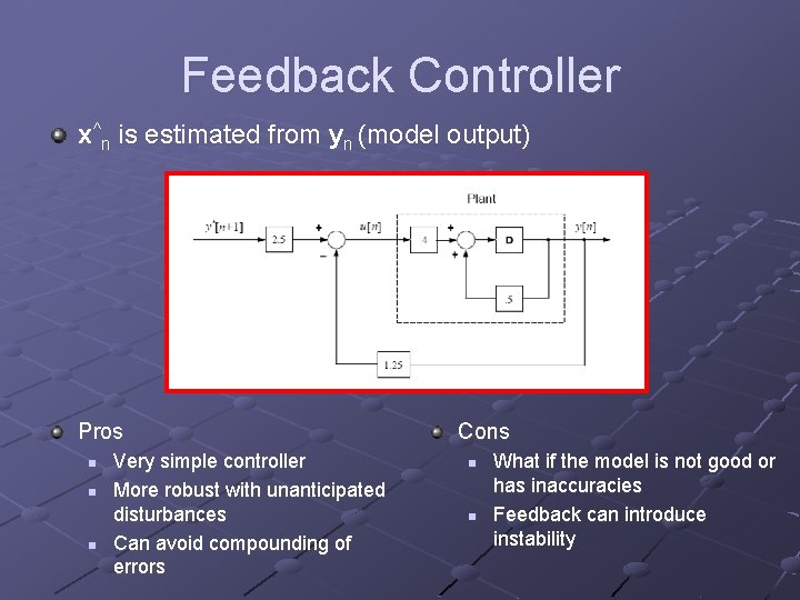
Feedback Controller x^n is estimated from yn (model output) Pros n n n Very simple controller More robust with unanticipated disturbances Can avoid compounding of errors Cons n n What if the model is not good or has inaccuracies Feedback can introduce instability

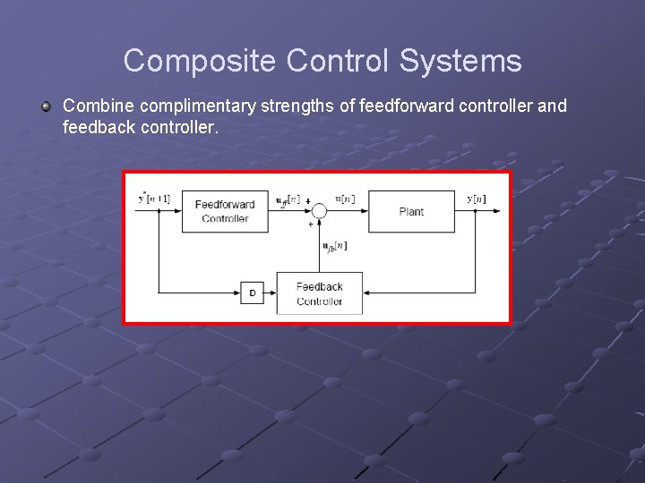
Composite Control Systems Combine complimentary strengths of feedforward controller and feedback controller.

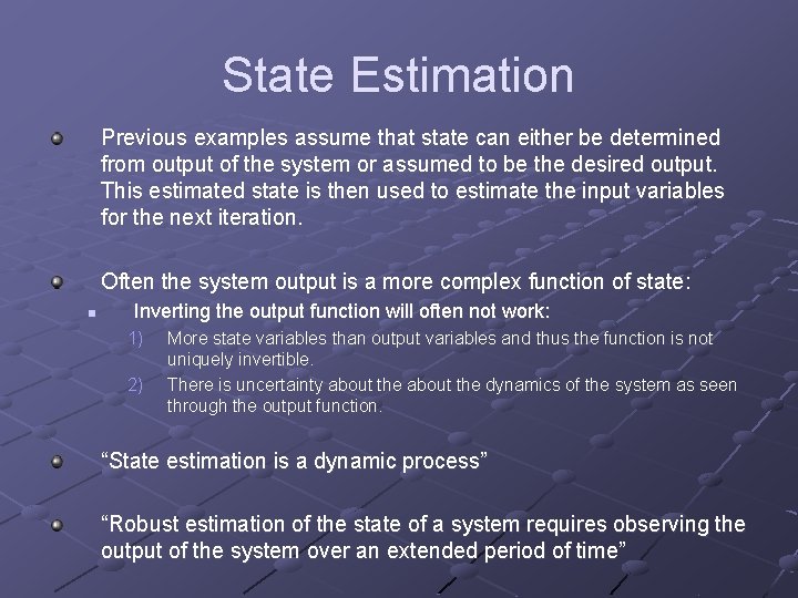
State Estimation Previous examples assume that state can either be determined from output of the system or assumed to be the desired output. This estimated state is then used to estimate the input variables for the next iteration. Often the system output is a more complex function of state: n Inverting the output function will often not work: 1) 2) More state variables than output variables and thus the function is not uniquely invertible. There is uncertainty about the dynamics of the system as seen through the output function. “State estimation is a dynamic process” “Robust estimation of the state of a system requires observing the output of the system over an extended period of time”

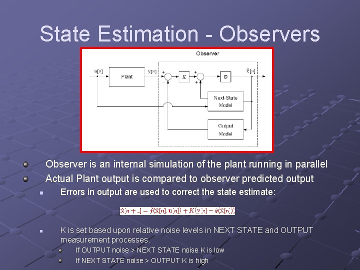
State Estimation - Observers Observer is an internal simulation of the plant running in parallel Actual Plant output is compared to observer predicted output n n Errors in output are used to correct the state estimate: K is set based upon relative noise levels in NEXT STATE and OUTPUT measurement processes. If OUTPUT noise > NEXT STATE noise K is low If NEXT STATE noise > OUTPUT K is high

Learning Algorithms Previous examples have dealt with systems and plants in relatively benign finite settings. Systems that need to interact with the real world will encounter situations or objects etc. that do not conform the system’s model. An adaptive process would allow the system to update its control mechanisms. Learning algorithms can be taught in two ways: 1) 2) Present whole gamut of available data prior to the deployment of the system or periodically update the learning algorithm Dynamically update control models after the presentation of each new piece of learning data. a. k. a On-Line Learning.

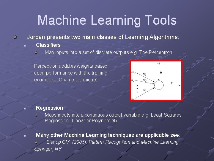
Machine Learning Tools Jordan presents two main classes of Learning Algorithms: n Classifiers Map inputs into a set of discrete outputs e. g. The Perceptron updates weights based upon performance with the training examples. (On-line technique) n Regression Maps inputs into a continuous output variable e. g. Least Squares Regression (Linear or Polynomial) n Many other Machine Learning techniques are applicable see: Bishop CM. (2006). Pattern Recognition and Machine Learning. Springer, NY

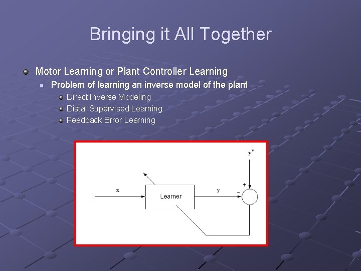
Bringing it All Together Motor Learning or Plant Controller Learning n Problem of learning an inverse model of the plant Direct Inverse Modeling Distal Supervised Learning Feedback Error Learning

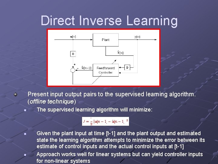
Direct Inverse Learning Present input output pairs to the supervised learning algorithm. (offline technique) n n n The supervised learning algorithm will minimize: Given the plant input at time [t-1] and the plant output and estimated state the learning algorithm attempts to minimize the error between its estimate of control inputs and the actual control inputs at [t-1] Approach works well for linear systems but can yield controller inputs for non-linear systems

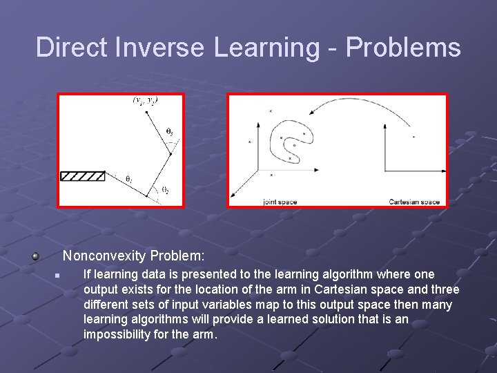
Direct Inverse Learning - Problems Nonconvexity Problem: n If learning data is presented to the learning algorithm where one output exists for the location of the arm in Cartesian space and three different sets of input variables map to this output space then many learning algorithms will provide a learned solution that is an impossibility for the arm.

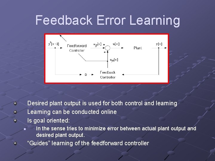
Feedback Error Learning Desired plant output is used for both control and learning Learning can be conducted online Is goal oriented: n In the sense tries to minimize error between actual plant output and desired plant output. “Guides” learning of the feedforward controller

Distal Supervised Learning Approach aims to solve the nonlinear model inverse problem as a composite system of forward plant model and feedforward controller model Two interactive processes used in learning the system n n Forward model is learned Forward model is used in the learning of the feedforward controller This approach avoids nonconvexity problem as the feedforward controller learns to minimize error.

Distal Supervised Learning II The Forward Model is trained using the prediction error: (y[n] - y^[n]). The composite learning system (Forward Model & Feedforward Controller) is trained using the performance error (y*[n] - y[n]). Where the Forward model is held fixed.

Conclusions Jordan presents a series of control architectures and control policy learning techniques Inverse and Forward models play complimentary roles n n n Inverse models are the basis for predictive control Forward models can be used to anticipate and cancel delayed feedback Basic blocks for dynamical state estimation When the models are learned using machine learning algorithms or techniques they provide capabilities for prediction, control and error correction that allow the system to cope with difficult nonlinear control problems “General rule…partial knowledge is better than no knowledge, if used appropriately”

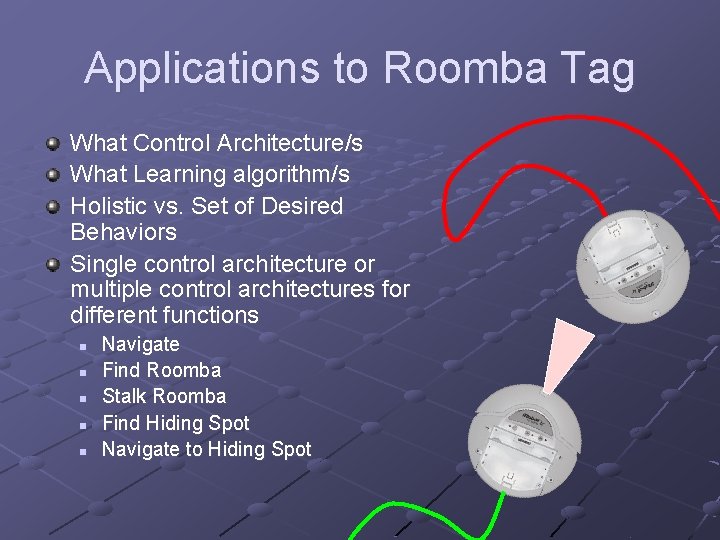
Applications to Roomba Tag What Control Architecture/s What Learning algorithm/s Holistic vs. Set of Desired Behaviors Single control architecture or multiple control architectures for different functions n n n Navigate Find Roomba Stalk Roomba Find Hiding Spot Navigate to Hiding Spot