CHAPTER 5 Risk and Return Past and Prologue

CHAPTER 5 Risk and Return: Past and Prologue

The Goals of Chapter 5 Introduce methods to calculate the holding period return (HRP, 持有期間收益率) Consider the inflation rate (通貨膨脹率) and real return (實質報酬率) Introduce the estimation of risk (the uncertainty of returns) and the risk premium (風險溢酬) – Show the historical return-risk patterns Asset allocation (資產配置) between the risky and riskless portfolios Introduce the capital market line (CML, 資本市 場線), which is the foundation of the CAPM (資 本資產定義理論) Supplement: Value at Risk (Va. R, 風險值) 5 -2

5. 1 RATES OF RETURN (報酬率) 5 -3

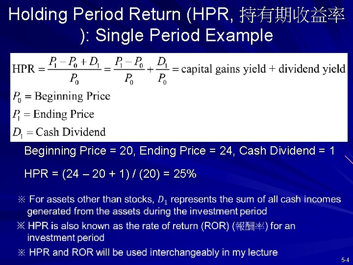
Holding Period Return (HPR, 持有期收益率 ): Single Period Example Beginning Price = 20, Ending Price = 24, Cash Dividend = 1 HPR = (24 – 20 + 1) / (20) = 25% 5 -4

Measuring Investment Returns Over Multiple Periods HPR is a simple and unambiguous measure of investment return over ONE period (單期HPR) However, investors are often interested in average returns over MULTIPLE periods (多期 平均報酬率) In this case, return measurement is more ambiguous, i. e. , there may be different methods to measure multi-period returns – Arithmetic average return (算術平均報酬率) – Geometric average return (幾何平均報酬率) – Dollar-weighted return (資金加權報酬率) 5 -5

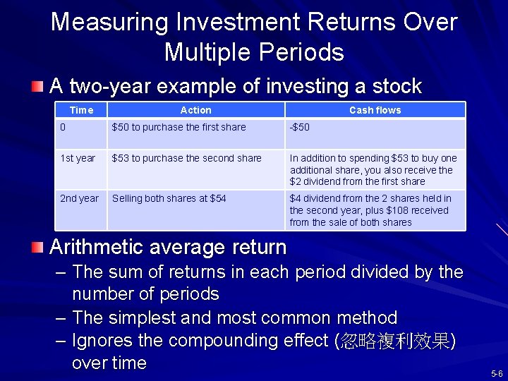
Measuring Investment Returns Over Multiple Periods A two-year example of investing a stock Time Action Cash flows 0 $50 to purchase the first share -$50 1 st year $53 to purchase the second share In addition to spending $53 to buy one additional share, you also receive the $2 dividend from the first share 2 nd year Selling both shares at $54 $4 dividend from the 2 shares held in the second year, plus $108 received from the sale of both shares Arithmetic average return – The sum of returns in each period divided by the number of periods – The simplest and most common method – Ignores the compounding effect (忽略複利效果) over time 5 -6

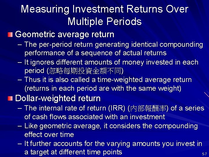
Measuring Investment Returns Over Multiple Periods Geometric average return – The per-period return generating identical compounding performance of a sequence of actual returns – It ignores different amounts of money invested in each period (忽略每期投資金額不同) – Thus it is also called a time-weighted average return (returns in each period are with the same weight) Dollar-weighted return – The internal rate of return (IRR) (內部報酬率) of a series of cash flows associated with an investment – Like geometric average, it considers the compounding effect over time – It further accounts for the varying amounts you invest in a target at different time points 5 -7

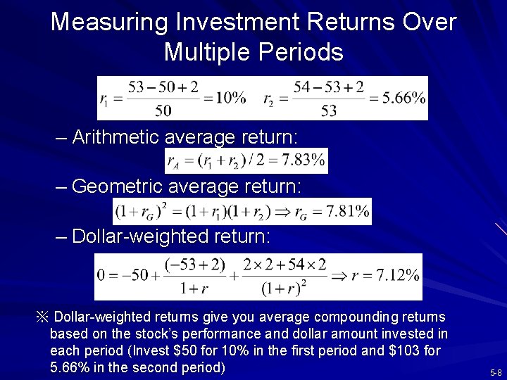
Measuring Investment Returns Over Multiple Periods – Arithmetic average return: – Geometric average return: – Dollar-weighted return: ※ Dollar-weighted returns give you average compounding returns based on the stock’s performance and dollar amount invested in each period (Invest $50 for 10% in the first period and $103 for 5. 66% in the second period) 5 -8

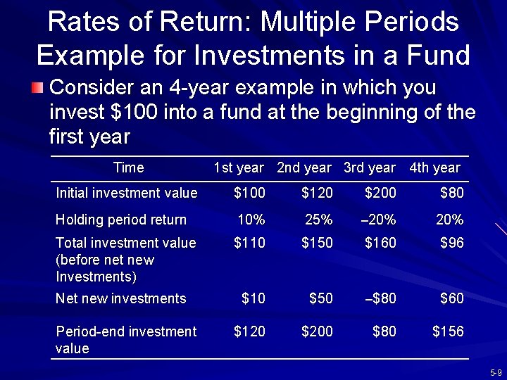
Rates of Return: Multiple Periods Example for Investments in a Fund Consider an 4 -year example in which you invest $100 into a fund at the beginning of the first year Time 1 st year 2 nd year 3 rd year 4 th year Initial investment value $100 $120 $200 $80 Holding period return 10% 25% – 20% Total investment value (before net new Investments) $110 $150 $160 $96 $10 $50 –$80 $60 $120 $200 $80 $156 Net new investments Period-end investment value 5 -9

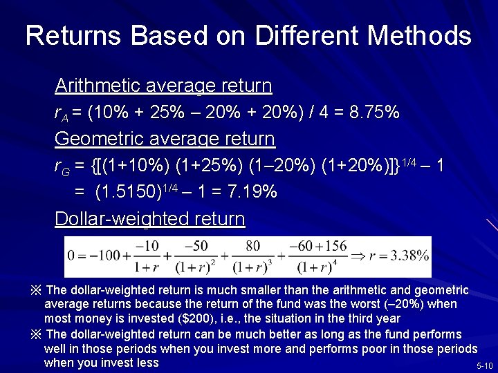
Returns Based on Different Methods Arithmetic average return r. A = (10% + 25% – 20% + 20%) / 4 = 8. 75% Geometric average return r. G = {[(1+10%) (1+25%) (1– 20%) (1+20%)]}1/4 – 1 = (1. 5150)1/4 – 1 = 7. 19% Dollar-weighted return ※ The dollar-weighted return is much smaller than the arithmetic and geometric average returns because the return of the fund was the worst (– 20%) when most money is invested ($200), i. e. , the situation in the third year ※ The dollar-weighted return can be much better as long as the fund performs well in those periods when you invest more and performs poor in those periods when you invest less 5 -10

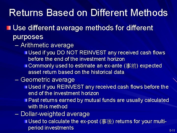
Returns Based on Different Methods Use different average methods for different purposes – Arithmetic average Used if you DO NOT REINVEST any received cash flows before the end of the investment horizon Commonly used to estimate an ex-ante (事前) expected asset return based on the historical data – Geometric average Used if you REINVEST any received cash flows before the end of the investment horizon Past returns earned by mutual funds are usually calculated with this method – Dollar-weighted average Used to calculate the ex-post (事後) returns for your multiperiod investments 5 -11

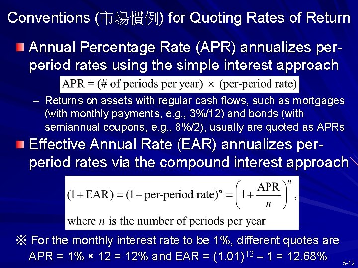
Conventions (市場慣例) for Quoting Rates of Return Annual Percentage Rate (APR) annualizes perperiod rates using the simple interest approach – Returns on assets with regular cash flows, such as mortgages (with monthly payments, e. g. , 3%/12) and bonds (with semiannual coupons, e. g. , 8%/2), usually are quoted as APRs Effective Annual Rate (EAR) annualizes perperiod rates via the compound interest approach ※ For the monthly interest rate to be 1%, different quotes are APR = 1% × 12 = 12% and EAR = (1. 01)12 – 1 = 12. 68% 5 -12

5. 2 INFLATION AND REAL RATES OF RETURN 5 -13

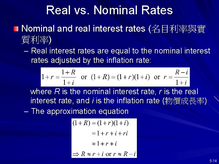
Real vs. Nominal Rates Nominal and real interest rates (名目利率與實 質利率) – Real interest rates are equal to the nominal interest rates adjusted by the inflation rate: where R is the nominal interest rate, r is the real interest rate, and i is the inflation rate (物價成長率) – The approximation equation 5 -14

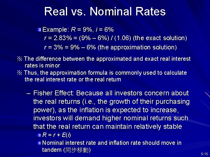
Real vs. Nominal Rates Example: R = 9%, i = 6% r = 2. 83% = (9% – 6%) / (1. 06) (the exact solution) r = 3% = 9% – 6% (the approximation solution) ※ The difference between the approximated and exact real interest rates is minor ※ Thus, the approximation formula is commonly used to calculate the real interest rate or the real return – Fisher Effect: Because all investors concern about the real returns (i. e. , the growth of their purchasing power), as the inflation is expected to increase, investors will demand higher nominal returns such that the real return can maintain relatively stable R = r + E (i ) Nominal interest rate and inflation rate should move in tandem (同步移動) 5 -15

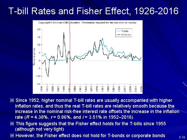
T-bill Rates and Fisher Effect, 1926 -2016 ※ Since 1952, higher nominal T-bill rates are usually accompanied with higher inflation rates, and thus the real T-bill rates are relatively smooth because the increase in the nominal risk-free interest rate offsets the increase in the inflation rate (R = 4. 38%, r = 0. 86%, and i = 3. 51% in 1952– 2016) ※ This figure suggests that the Fisher effect holds for the T-bills since 1955 (although not very tight) ※ However, the Fisher effect does not hold for T-bonds or corporate bonds 5 -16

5. 3 RISK AND RISK PREMIUMS (風險與風險溢酬) 5 -17

Risk Definition: the uncertainty about future holding period returns (風險是未來持有期間收益率的不 確定性) for an investment – This definition of risk is the most common and classical assumption in finance and economics – Risk is NOT how much you could LOSE from the investment (風險並非投資的可能損失) – As long as the realized returns deviate from your expectation, it is risk ※ At the end of this chapter, another definition of risk, Value at Risk (Va. R, 風險值), which considers possible losses given a probability level as risk, is introduced 5 -18

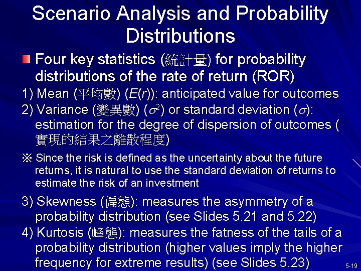
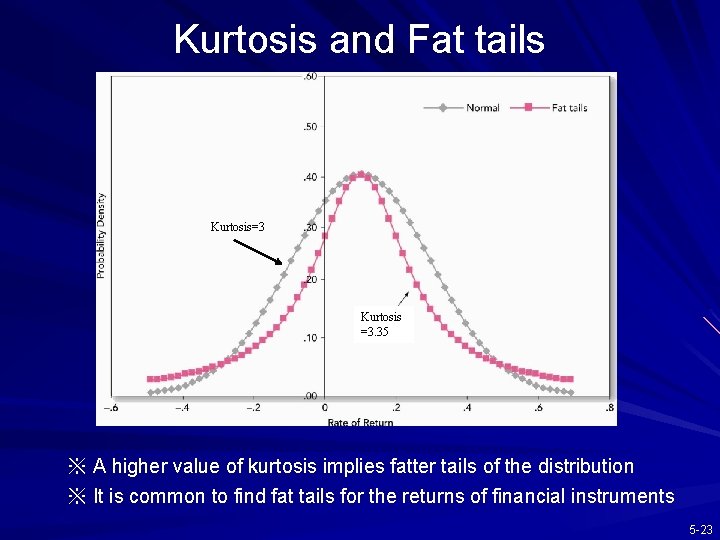
Scenario Analysis and Probability Distributions Four key statistics (統計量) for probability distributions of the rate of return (ROR) 1) Mean (平均數) (E(r)): anticipated value for outcomes 2) Variance (變異數) ( 2) or standard deviation ( ): estimation for the degree of dispersion of outcomes ( 實現的結果之離散程度) ※ Since the risk is defined as the uncertainty about the future returns, it is natural to use the standard deviation of returns to estimate the risk of an investment 3) Skewness (偏態): measures the asymmetry of a probability distribution (see Slides 5. 21 and 5. 22) 4) Kurtosis (峰態): measures the fatness of the tails of a probability distribution (higher values imply the higher frequency for extreme results) (see Slides 5. 23) 5 -19

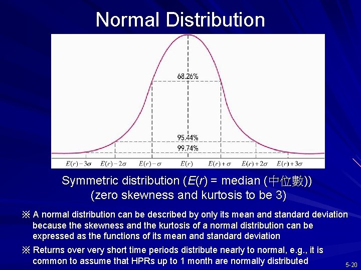
Normal Distribution Symmetric distribution (E(r) = median (中位數)) (zero skewness and kurtosis to be 3) ※ A normal distribution can be described by only its mean and standard deviation because the skewness and the kurtosis of a normal distribution can be expressed as the functions of its mean and standard deviation ※ Returns over very short time periods distribute nearly to normal, e. g. , it is common to assume that HPRs up to 1 month are normally distributed 5 -20

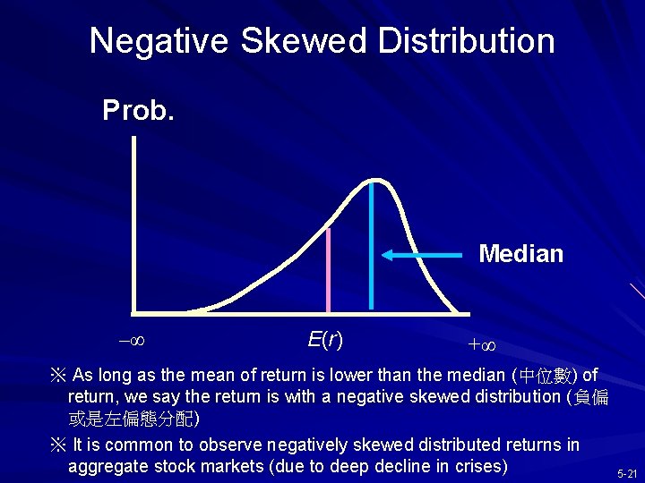
Negative Skewed Distribution Prob. Median –∞ E(r) +∞ ※ As long as the mean of return is lower than the median (中位數) of return, we say the return is with a negative skewed distribution (負偏 或是左偏態分配) ※ It is common to observe negatively skewed distributed returns in aggregate stock markets (due to deep decline in crises) 5 -21

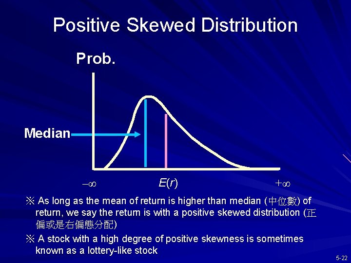
Positive Skewed Distribution Prob. Median –∞ E(r) +∞ ※ As long as the mean of return is higher than median (中位數) of return, we say the return is with a positive skewed distribution (正 偏或是右偏態分配) ※ A stock with a high degree of positive skewness is sometimes known as a lottery-like stock 5 -22

Kurtosis and Fat tails Kurtosis=3 Kurtosis =3. 35 ※ A higher value of kurtosis implies fatter tails of the distribution ※ It is common to find fat tails for the returns of financial instruments 5 -23

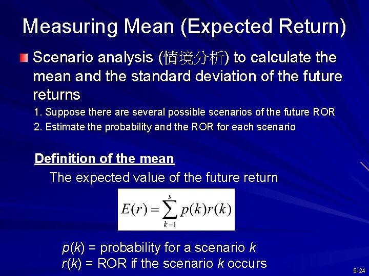
Measuring Mean (Expected Return) Scenario analysis (情境分析) to calculate the mean and the standard deviation of the future returns 1. Suppose there are several possible scenarios of the future ROR 2. Estimate the probability and the ROR for each scenario Definition of the mean The expected value of the future return p(k) = probability for a scenario k r(k) = ROR if the scenario k occurs 5 -24

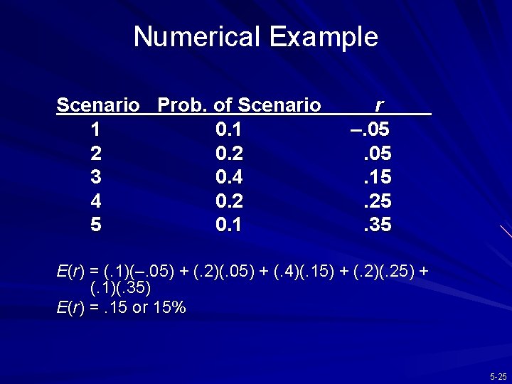
Numerical Example Scenario Prob. of Scenario 1 0. 1 2 0. 2 3 0. 4 4 0. 2 5 0. 1 r –. 05. 15. 25. 35 E(r) = (. 1)(–. 05) + (. 2)(. 05) + (. 4)(. 15) + (. 2)(. 25) + (. 1)(. 35) E(r) =. 15 or 15% 5 -25

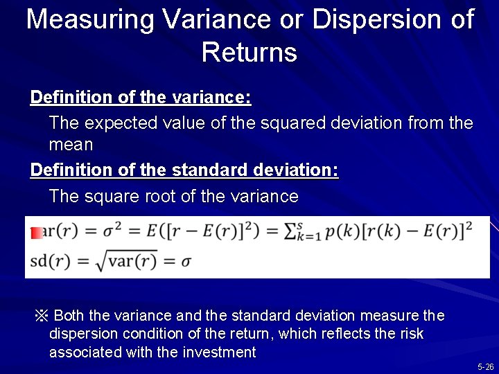
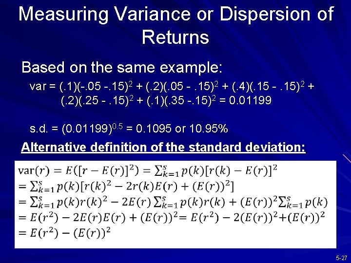
Measuring Variance or Dispersion of Returns Definition of the variance: The expected value of the squared deviation from the mean Definition of the standard deviation: The square root of the variance ※ Both the variance and the standard deviation measure the dispersion condition of the return, which reflects the risk associated with the investment 5 -26

Measuring Variance or Dispersion of Returns Based on the same example: var = (. 1)(-. 05 -. 15)2 + (. 2)(. 05 -. 15)2 + (. 4)(. 15 -. 15)2 + (. 2)(. 25 -. 15)2 + (. 1)(. 35 -. 15)2 = 0. 01199 s. d. = (0. 01199)0. 5 = 0. 1095 or 10. 95% Alternative definition of the standard deviation: 5 -27

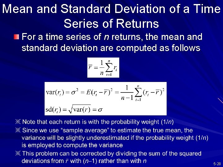
Mean and Standard Deviation of a Time Series of Returns For a time series of n returns, the mean and standard deviation are computed as follows 5 -28

Risk Premiums and Risk Aversion Denote rf and r. P as the HPRs of the risk-free asset and a risky portfolio, respectively – The excess return (超額報酬) of the risky portfolio is the rate of return in excess of rf, i. e. , r. P – rf – The risk premium (風險溢酬) of that portfolio is the EXPECTED excess return, i. e. , E(r. P) – rf ※ It is common to use the HPR of T-bills to be the risk-free interest rate rf ※ For the risk premium: there is no expectation for rf because the HPR of Tbills is known at the beginning of the holding period, but we cannot know the HPR of the risky portfolio r. P until the end of the holding period ※ The name of risk premium: if you would like to bear some risk, you can earn the premium corresponding to that risk on average ※ It is common to estimate E(r. P) from the series of historical returns ※ However, note that the return of T-bills also varies for each period, so in practice we usually estimate the risk premium as a whole directly by calculating the average of historical excess returns 5 -29

Risk Premiums and Risk Aversion Risk aversion is the degree of the reluctance of a person to accept risk, i. e. , risk averse investors do not like the uncertainty of the return of their investment Risk averse (風險趨避) vs. Risk neutral (風險 中立) vs. Risk loving (風險愛好) The risk averse attitude is reflected by the phenomenon that investors require higher risk premium for assets with higher risk For a more risk averse investor, he needs higher risk premium to attract him to invest in a risky portfolio 5 -30

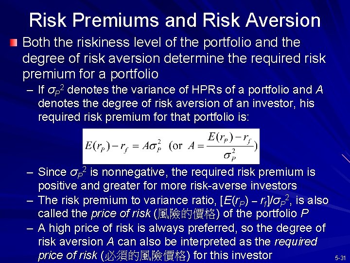
Risk Premiums and Risk Aversion Both the riskiness level of the portfolio and the degree of risk aversion determine the required risk premium for a portfolio – If σP 2 denotes the variance of HPRs of a portfolio and A denotes the degree of risk aversion of an investor, his required risk premium for that portfolio is: – Since σP 2 is nonnegative, the required risk premium is positive and greater for more risk-averse investors – The risk premium to variance ratio, [E(r. P) – rf]/σP 2, is also called the price of risk (風險的價格) of the portfolio P – A high price of risk is always preferred, so the degree of risk aversion A can also be interpreted as the required price of risk (必須的風險價格) for this investor 5 -31

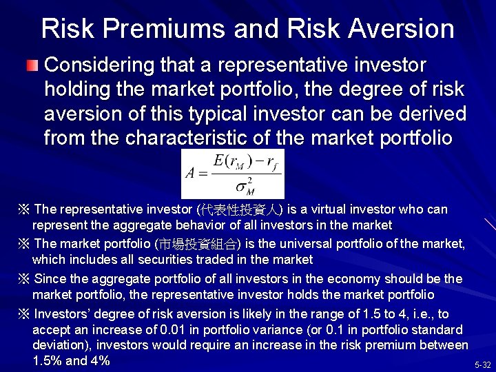
Risk Premiums and Risk Aversion Considering that a representative investor holding the market portfolio, the degree of risk aversion of this typical investor can be derived from the characteristic of the market portfolio ※ The representative investor (代表性投資人) is a virtual investor who can represent the aggregate behavior of all investors in the market ※ The market portfolio (市場投資組合) is the universal portfolio of the market, which includes all securities traded in the market ※ Since the aggregate portfolio of all investors in the economy should be the market portfolio, the representative investor holds the market portfolio ※ Investors’ degree of risk aversion is likely in the range of 1. 5 to 4, i. e. , to accept an increase of 0. 01 in portfolio variance (or 0. 1 in portfolio standard deviation), investors would require an increase in the risk premium between 1. 5% and 4% 5 -32

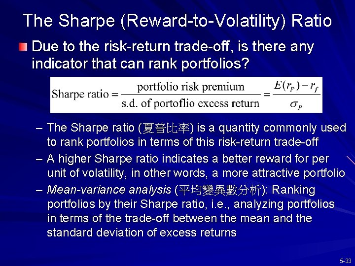
The Sharpe (Reward-to-Volatility) Ratio Due to the risk-return trade-off, is there any indicator that can rank portfolios? – The Sharpe ratio (夏普比率) is a quantity commonly used to rank portfolios in terms of this risk-return trade-off – A higher Sharpe ratio indicates a better reward for per unit of volatility, in other words, a more attractive portfolio – Mean-variance analysis (平均變異數分析): Ranking portfolios by their Sharpe ratio, i. e. , analyzing portfolios in terms of the trade-off between the mean and the standard deviation of excess returns 5 -33

5. 4 THE HISTORICAL RECORD 5 -34

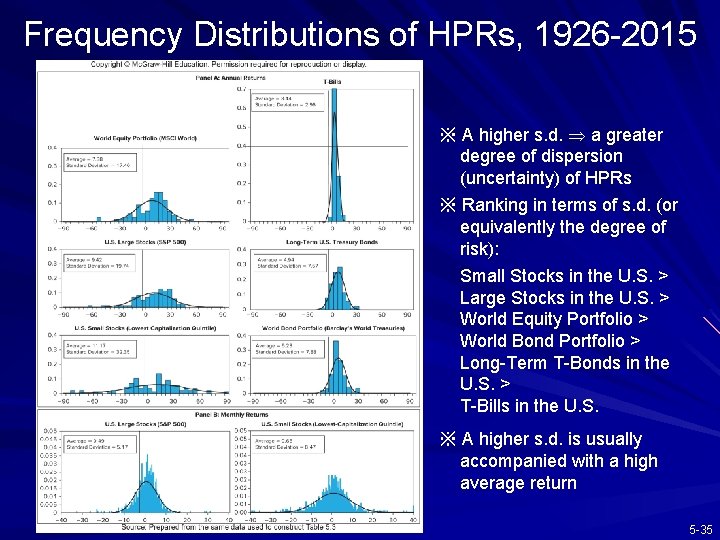
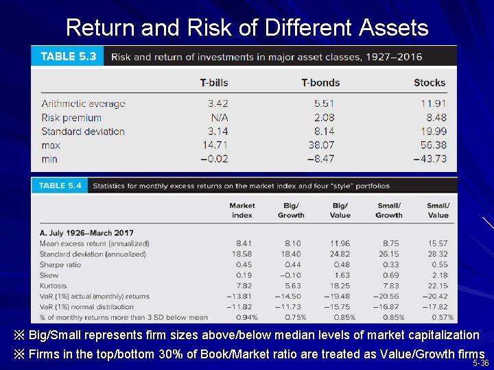
Frequency Distributions of HPRs, 1926 -2015 ※ A higher s. d. a greater degree of dispersion (uncertainty) of HPRs ※ Ranking in terms of s. d. (or equivalently the degree of risk): Small Stocks in the U. S. > Large Stocks in the U. S. > World Equity Portfolio > World Bond Portfolio > Long-Term T-Bonds in the U. S. > T-Bills in the U. S. ※ A higher s. d. is usually accompanied with a high average return 5 -35

Return and Risk of Different Assets ※ Big/Small represents firm sizes above/below median levels of market capitalization ※ Firms in the top/bottom 30% of Book/Market ratio are treated as Value/Growth firms 5 -36

5. 5 ASSET ALLOCATION ACROSS RISKY PORTFOLIOS AND THE RISK-FREE ASSET 5 -37

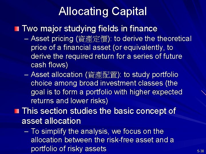
Allocating Capital Two major studying fields in finance – Asset pricing (資產定價): to derive theoretical price of a financial asset (or equivalently, to derive the required return for a series of future cash flows) – Asset allocation (資產配置): to study portfolio choice among broad investment classes (the goal is to form a portfolio with higher expected returns and lower risks) This section studies the basic concept of asset allocation – To simplify the analysis, we focus on the allocation between the risk-free asset and a portfolio of risky assets 5 -38

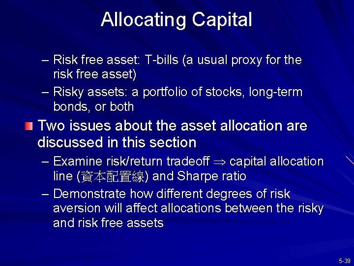
Allocating Capital – Risk free asset: T-bills (a usual proxy for the risk free asset) – Risky assets: a portfolio of stocks, long-term bonds, or both Two issues about the asset allocation are discussed in this section – Examine risk/return tradeoff capital allocation line (資本配置線) and Sharpe ratio – Demonstrate how different degrees of risk aversion will affect allocations between the risky and risk free assets 5 -39

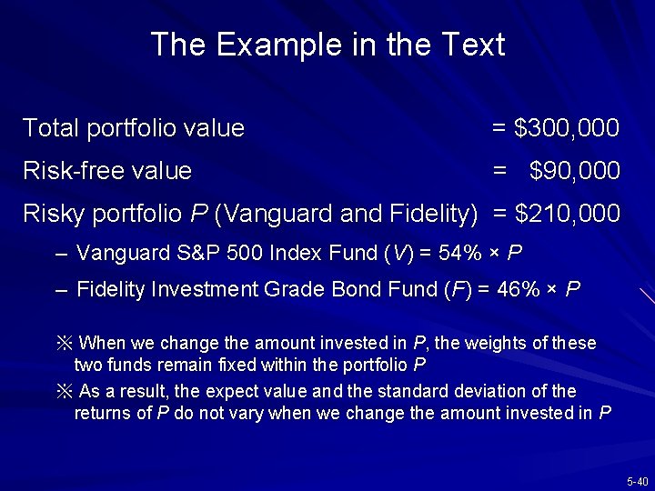
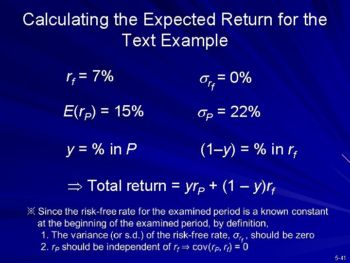
The Example in the Text Total portfolio value = $300, 000 Risk-free value = $90, 000 Risky portfolio P (Vanguard and Fidelity) = $210, 000 – Vanguard S&P 500 Index Fund (V) = 54% × P – Fidelity Investment Grade Bond Fund (F) = 46% × P ※ When we change the amount invested in P, the weights of these two funds remain fixed within the portfolio P ※ As a result, the expect value and the standard deviation of the returns of P do not vary when we change the amount invested in P 5 -40

Calculating the Expected Return for the Text Example rf = 7% rf = 0% E(r. P) = 15% P = 22% y = % in P (1–y) = % in rf Total return = yr. P + (1 – y)rf 5 -41

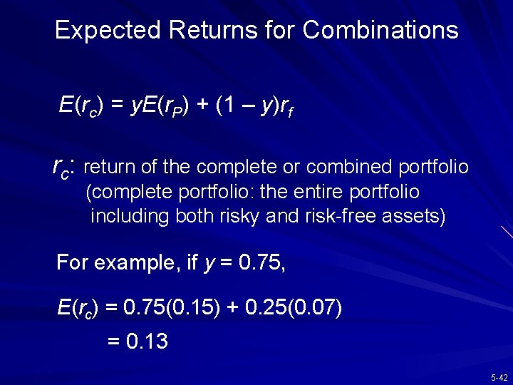
Expected Returns for Combinations E(rc) = y. E(r. P) + (1 – y)rf rc: return of the complete or combined portfolio (complete portfolio: the entire portfolio including both risky and risk-free assets) For example, if y = 0. 75, E(rc) = 0. 75(0. 15) + 0. 25(0. 07) = 0. 13 5 -42

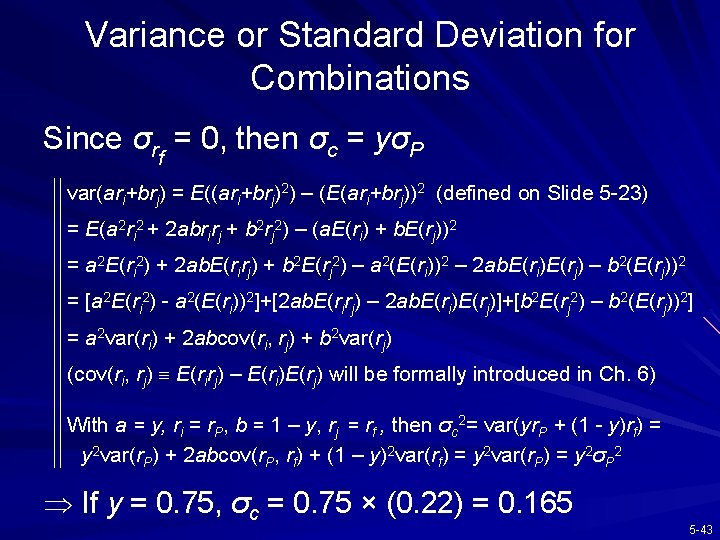
Variance or Standard Deviation for Combinations Since σrf = 0, then σc = yσP var(ari+brj) = E((ari+brj)2) – (E(ari+brj))2 (defined on Slide 5 -23) = E(a 2 ri 2 + 2 abrirj + b 2 rj 2) – (a. E(ri) + b. E(rj))2 = a 2 E(ri 2) + 2 ab. E(rirj) + b 2 E(rj 2) – a 2(E(ri))2 – 2 ab. E(ri)E(rj) – b 2(E(rj))2 = [a 2 E(ri 2) - a 2(E(ri))2]+[2 ab. E(rirj) – 2 ab. E(ri)E(rj)]+[b 2 E(rj 2) – b 2(E(rj))2] = a 2 var(ri) + 2 abcov(ri, rj) + b 2 var(rj) (cov(ri, rj) E(rirj) – E(ri)E(rj) will be formally introduced in Ch. 6) With a = y, ri = r. P, b = 1 – y, rj = rf , then σc 2= var(yr. P + (1 - y)rf) = y 2 var(r. P) + 2 abcov(r. P, rf) + (1 – y)2 var(rf) = y 2 var(r. P) = y 2σP 2 If y = 0. 75, σc = 0. 75 × (0. 22) = 0. 165 5 -43

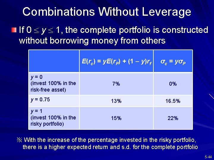
Combinations Without Leverage If 0 y 1, the complete portfolio is constructed without borrowing money from others E(rc) = y. E(r. P) + (1 – y)rf σ c = yσ P y=0 (invest 100% in the risk-free asset) 7% 0% y = 0. 75 13% 16. 5% y=1 (invest 100% in the risky portfolio) 15% 22% ※ With the increase of the percentage invested in the risky portfolio, there is a higher expected return and s. d. for the complete portfolio 5 -44

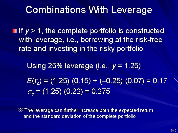
Combinations With Leverage If y > 1, the complete portfolio is constructed with leverage, i. e. , borrowing at the risk-free rate and investing in the risky portfolio Using 25% leverage (i. e. , y = 1. 25) E(rc) = (1. 25) (0. 15) + (– 0. 25) (0. 07) = 0. 17 c = (1. 25) (0. 22) = 0. 275 ※ The leverage can further increase both the expected return and the standard deviation of the complete portfolio 5 -45

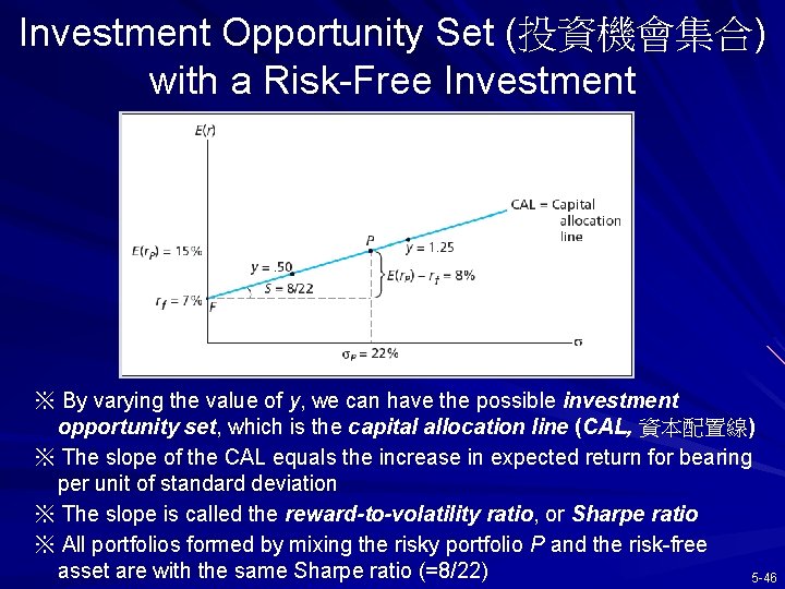
Investment Opportunity Set (投資機會集合) with a Risk-Free Investment ※ By varying the value of y, we can have the possible investment opportunity set, which is the capital allocation line (CAL, 資本配置線) ※ The slope of the CAL equals the increase in expected return for bearing per unit of standard deviation ※ The slope is called the reward-to-volatility ratio, or Sharpe ratio ※ All portfolios formed by mixing the risky portfolio P and the risk-free asset are with the same Sharpe ratio (=8/22) 5 -46

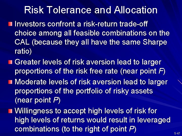
Risk Tolerance and Allocation Investors confront a risk-return trade-off choice among all feasible combinations on the CAL (because they all have the same Sharpe ratio) Greater levels of risk aversion lead to larger proportions of the risk free rate (near point F) Moderate levels of risk aversion lead to larger proportions of the portfolio of risky assets (near point P) Willingness to accept high levels of risk for high levels of returns would result in leveraged combinations (to the right of point P) 5 -47

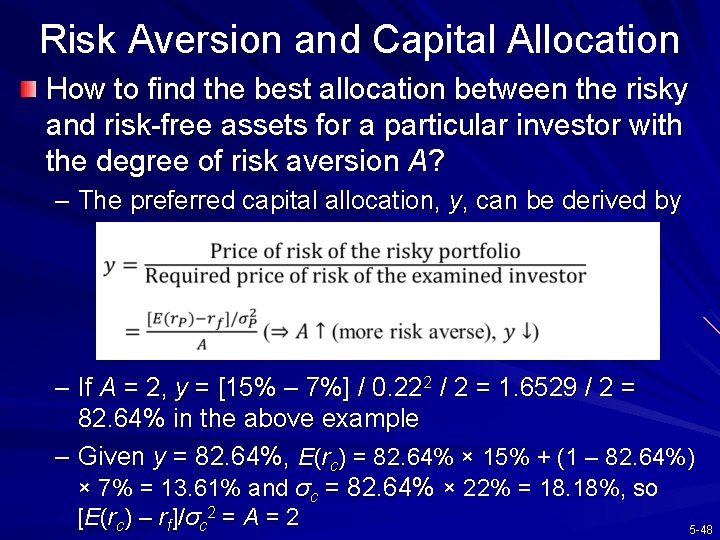
Risk Aversion and Capital Allocation How to find the best allocation between the risky and risk-free assets for a particular investor with the degree of risk aversion A? – The preferred capital allocation, y, can be derived by – If A = 2, y = [15% – 7%] / 0. 222 / 2 = 1. 6529 / 2 = 82. 64% in the above example – Given y = 82. 64%, E(rc) = 82. 64% × 15% + (1 – 82. 64%) × 7% = 13. 61% and σc = 82. 64% × 22% = 18. 18%, so [E(rc) – rf]/σc 2 = A = 2 5 -48

5. 6 PASSIVE STRATEGIES AND THE CAPITAL MARKET LINE 5 -49

Costs and Benefits of Passive Investing Investors can choose the assets included in the risky portfolio using passive or active strategies – Active strategy entails both costs on security analysis and on trading transaction – Passive strategy is based on the premise that most securities are fairly priced, so it selects a diversified portfolio of common stocks It is common to invest in an index fund which requires the least effort to manage the portfolio and thus the lowest operating expenses among all mutual stock funds 5 -50

Costs and Benefits of Passive Investing Free-rider (免費享用者) benefit: If there are many active, knowledgeable investors who quickly bid up prices of undervalued assets and offer down overvalued assets, most of the time most assets are fairly priced – Therefore, the performance of the passive strategy may not be inferior to that of the active strategy 5 -51

Costs and Benefits of Passive Investing The combined portfolio based on the passive strategy – Short-term T-bills – Portfolio of common stocks that mirrors the stock market portfolio We call the capital allocation line (CAL) provided by one-month T-bills (the risk-free asset) and a market-index portfolio (the risky asset) capital market line (CML, 資本市場線) 5 -52

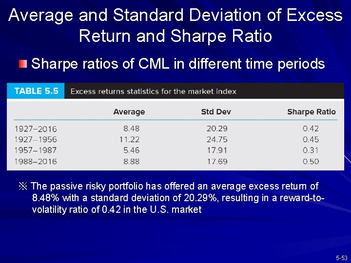
Average and Standard Deviation of Excess Return and Sharpe Ratio Sharpe ratios of CML in different time periods ※ The passive risky portfolio has offered an average excess return of 8. 48% with a standard deviation of 20. 29%, resulting in a reward-tovolatility ratio of 0. 42 in the U. S. market 5 -53

Value at Risk (Va. R) (風險值) 5 -54

Value at Risk (Va. R) Va. R (風險值) attempts to answer – The maximum possible amount to lose on a given portfolio at a specified level of probability The typical specified probability level is 5%, i. e. , to find the critical HPR (that is Va. R) corresponding to the worst 5% probability The probability that the loss exceeds Va. R is less than 5% Va. R is another measure of risk and measures losses that will be suffered given an extreme, adverse, price change – If returns are normally distributed, a function in Excel can be employed to determine how many standard deviations below the mean represents a 5% cumulative probability from the negative infinity: Norminv (0. 05, 0, 1) = – 1. 64485 standard deviations 5 -55

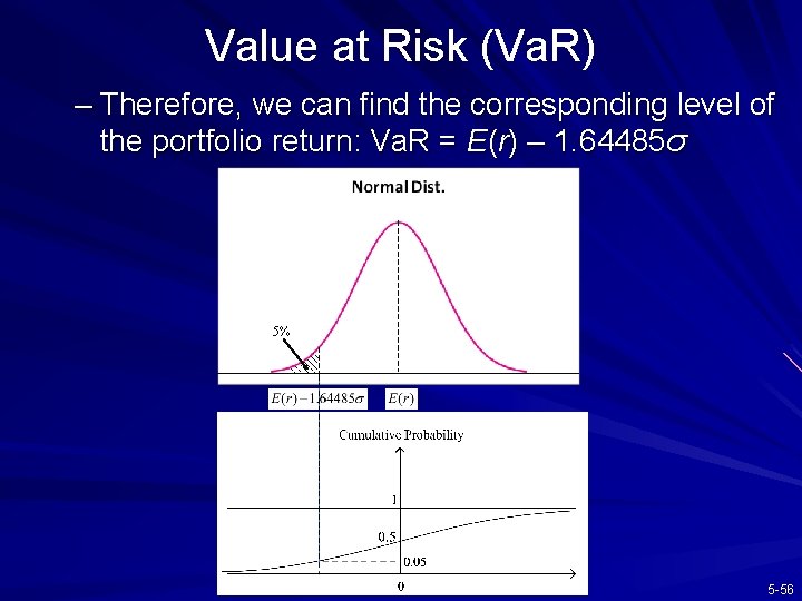
Value at Risk (Va. R) – Therefore, we can find the corresponding level of the portfolio return: Va. R = E(r) – 1. 64485σ 5% 5 -56

Value at Risk (Va. R) – A $500, 000 stock portfolio has an annual expected return of 12% and a standard deviation of 35%. What is the portfolio Va. R at a 5% probability level? Va. R = 12% – 1. 64485 × 35% = – 45. 57% Va. R$ = $500, 000 × – 45. 57% = –$227, 850 ※The probability for the losses larger than $227, 850 is smaller than 5% (or said there is 95% that the maximum losses will not exceed $227, 850) 5 -57

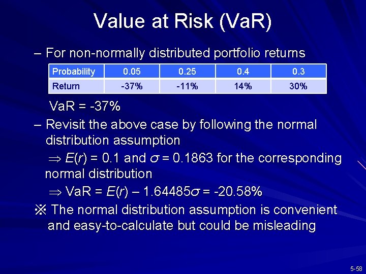
Value at Risk (Va. R) – For non-normally distributed portfolio returns Probability 0. 05 0. 25 0. 4 0. 3 Return -37% -11% 14% 30% Va. R = -37% – Revisit the above case by following the normal distribution assumption E(r) = 0. 1 and σ = 0. 1863 for the corresponding normal distribution Va. R = E(r) – 1. 64485σ = -20. 58% ※ The normal distribution assumption is convenient and easy-to-calculate but could be misleading 5 -58