Chapter 11 Risk and Return in Capital Markets

Chapter 11 Risk and Return in Capital Markets

Chapter Outline 11. 1 A First Look at Risk and Return 11. 2 Historical Risks and Returns of Stocks 11. 3 The Historical Tradeoff Between Risk and Return 11. 4 Common Versus Independent Risk 11. 5 Diversification in Stock Portfolios 2

Learning Objectives Identify which types of securities have historically had the highest returns and which have been the most volatile Compute the average return and volatility of returns from a set of historical asset prices Understand the tradeoff between risk and return for large portfolios versus individual stocks Describe the difference between common and independent risk Explain how diversified portfolios remove independent risk, leaving common risk as the only risk requiring a risk premium 3

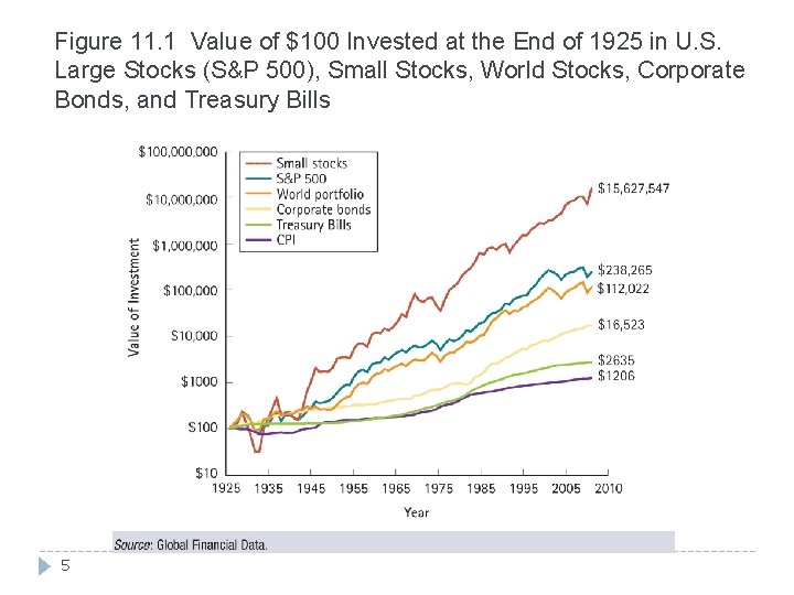
11. 1 A First Look at Risk and Return Consider how an investment would have grown if it were invested in each of the following from the end of 1925 until the beginning of 2010: Standard & Poor’s 500 (S&P 500) Small Stocks World Portfolio Corporate Bonds Treasury Bills 4

Figure 11. 1 Value of $100 Invested at the End of 1925 in U. S. Large Stocks (S&P 500), Small Stocks, World Stocks, Corporate Bonds, and Treasury Bills 5

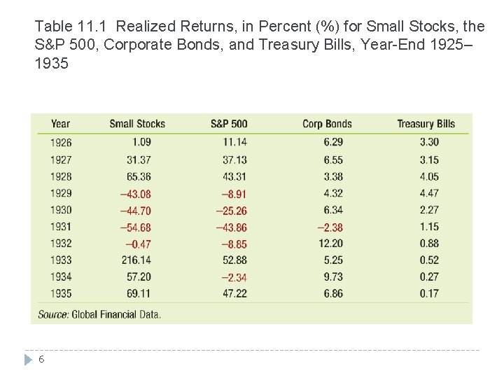
Table 11. 1 Realized Returns, in Percent (%) for Small Stocks, the S&P 500, Corporate Bonds, and Treasury Bills, Year-End 1925– 1935 6

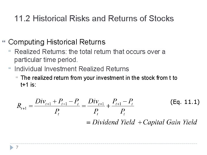
11. 2 Historical Risks and Returns of Stocks Computing Historical Returns Realized Returns: the total return that occurs over a particular time period. Individual Investment Realized Returns The realized return from your investment in the stock from t to t+1 is: (Eq. 11. 1) 7

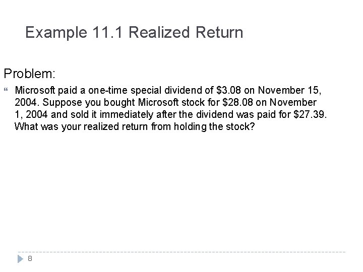
Example 11. 1 Realized Return Problem: Microsoft paid a one-time special dividend of $3. 08 on November 15, 2004. Suppose you bought Microsoft stock for $28. 08 on November 1, 2004 and sold it immediately after the dividend was paid for $27. 39. What was your realized return from holding the stock? 8

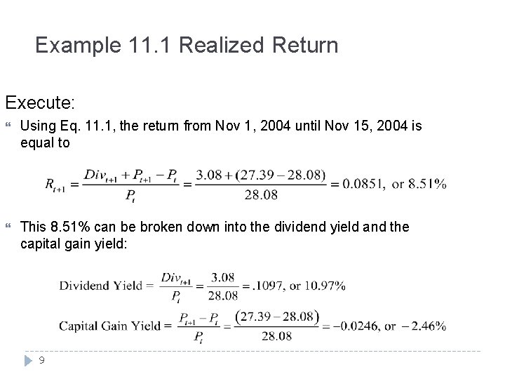
Example 11. 1 Realized Return Execute: Using Eq. 11. 1, the return from Nov 1, 2004 until Nov 15, 2004 is equal to This 8. 51% can be broken down into the dividend yield and the capital gain yield: 9

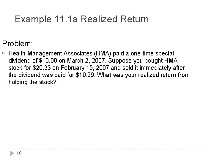
Example 11. 1 a Realized Return Problem: Health Management Associates (HMA) paid a one-time special dividend of $10. 00 on March 2, 2007. Suppose you bought HMA stock for $20. 33 on February 15, 2007 and sold it immediately after the dividend was paid for $10. 29. What was your realized return from holding the stock? 10

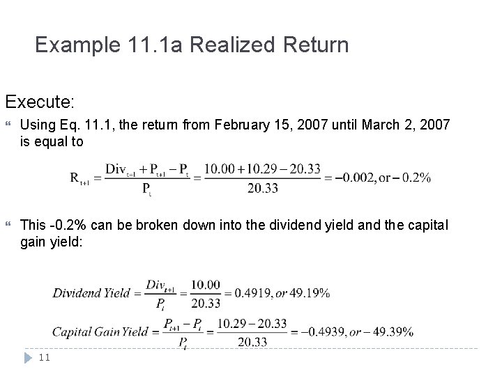
Example 11. 1 a Realized Return Execute: Using Eq. 11. 1, the return from February 15, 2007 until March 2, 2007 is equal to This -0. 2% can be broken down into the dividend yield and the capital gain yield: 11

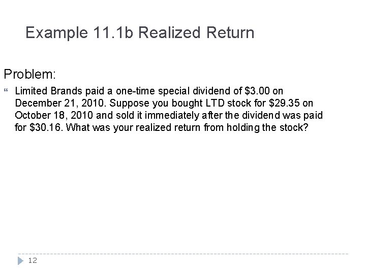
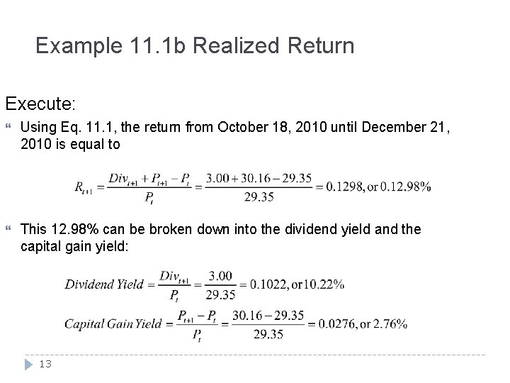
Example 11. 1 b Realized Return Problem: Limited Brands paid a one-time special dividend of $3. 00 on December 21, 2010. Suppose you bought LTD stock for $29. 35 on October 18, 2010 and sold it immediately after the dividend was paid for $30. 16. What was your realized return from holding the stock? 12

Example 11. 1 b Realized Return Execute: Using Eq. 11. 1, the return from October 18, 2010 until December 21, 2010 is equal to This 12. 98% can be broken down into the dividend yield and the capital gain yield: 13

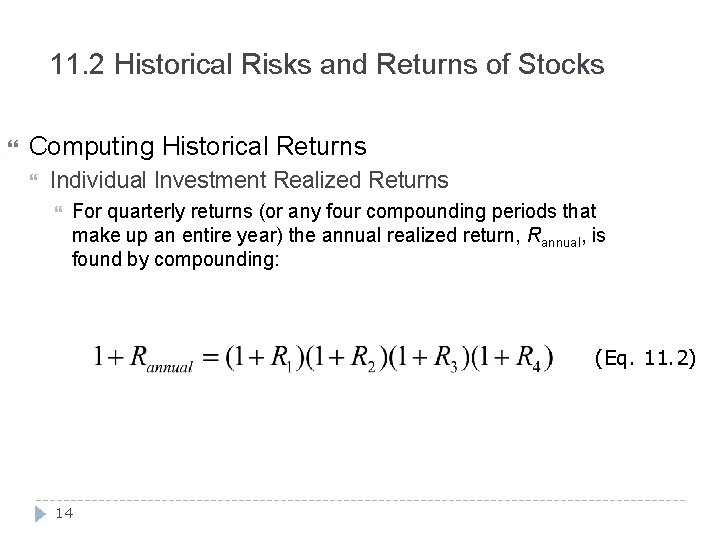
11. 2 Historical Risks and Returns of Stocks Computing Historical Returns Individual Investment Realized Returns For quarterly returns (or any four compounding periods that make up an entire year) the annual realized return, Rannual, is found by compounding: (Eq. 11. 2) 14

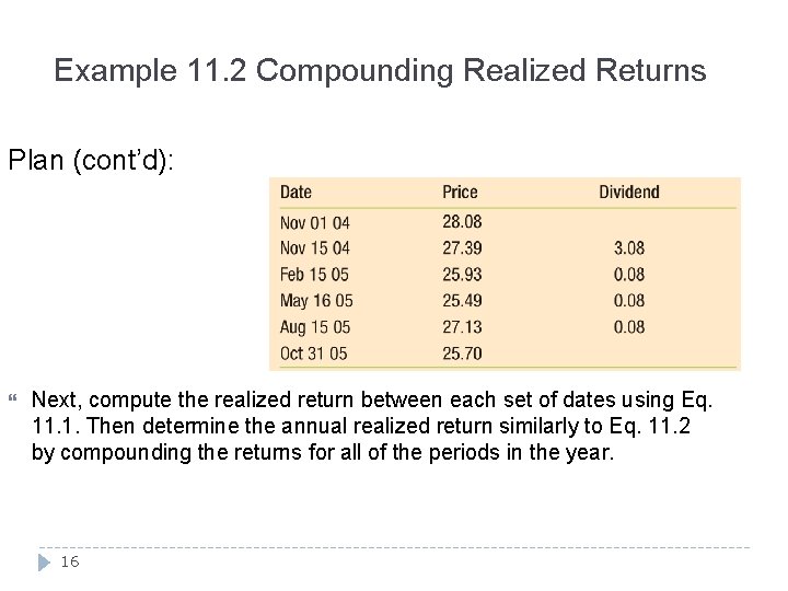
Example 11. 2 Compounding Realized Returns Problem: Suppose you purchased Microsoft stock (MSFT) on Nov 1, 2004 and held it for one year, selling on Oct 31, 2005. What was your annual realized return? 15

Example 11. 2 Compounding Realized Returns Plan (cont’d): Next, compute the realized return between each set of dates using Eq. 11. 1. Then determine the annual realized return similarly to Eq. 11. 2 by compounding the returns for all of the periods in the year. 16

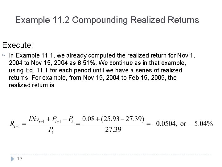
Example 11. 2 Compounding Realized Returns Execute: In Example 11. 1, we already computed the realized return for Nov 1, 2004 to Nov 15, 2004 as 8. 51%. We continue as in that example, using Eq. 11. 1 for each period until we have a series of realized returns. For example, from Nov 15, 2004 to Feb 15, 2005, the realized return is 17

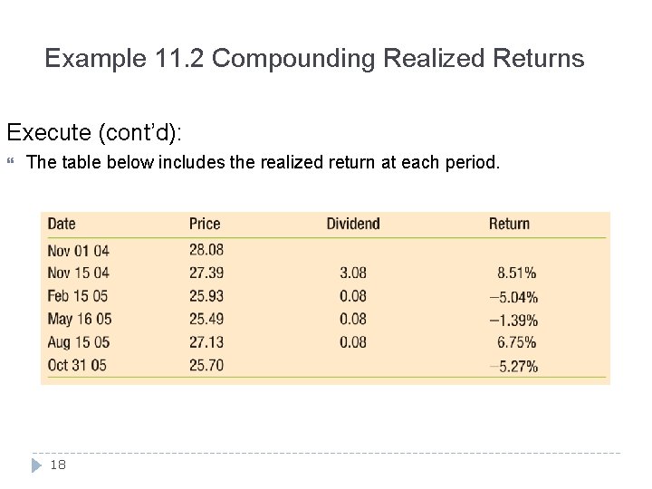
Example 11. 2 Compounding Realized Returns Execute (cont’d): The table below includes the realized return at each period. 18

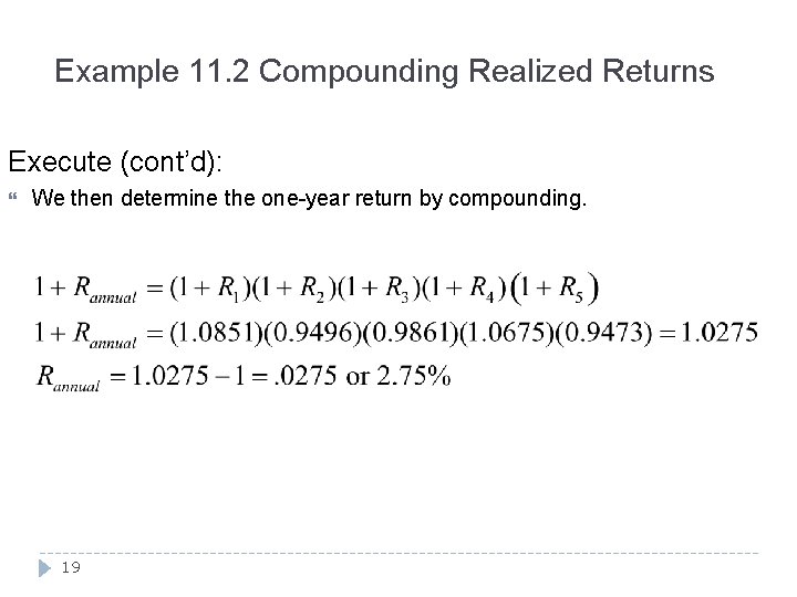
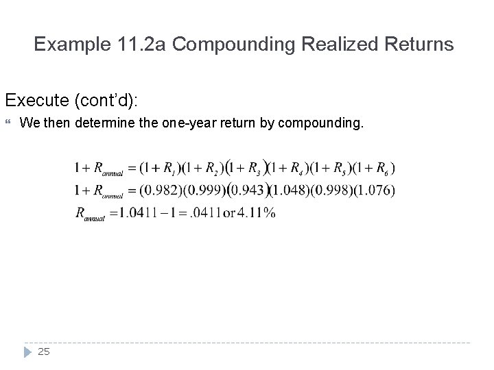
Example 11. 2 Compounding Realized Returns Execute (cont’d): We then determine the one-year return by compounding. 19

Example 11. 2 Compounding Realized Returns Evaluate: By repeating these steps, we have successfully computed the realized annual returns for an investor holding MSFT stock over this one-year period. From this exercise we can see that returns are risky. MSFT fluctuated up and down over the year and ended-up only slightly (2. 75%) at the end. 20

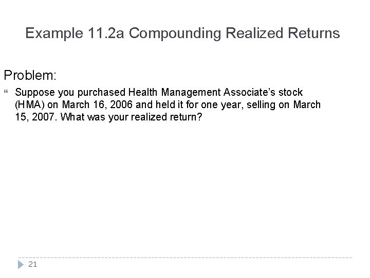
Example 11. 2 a Compounding Realized Returns Problem: Suppose you purchased Health Management Associate’s stock (HMA) on March 16, 2006 and held it for one year, selling on March 15, 2007. What was your realized return? 21

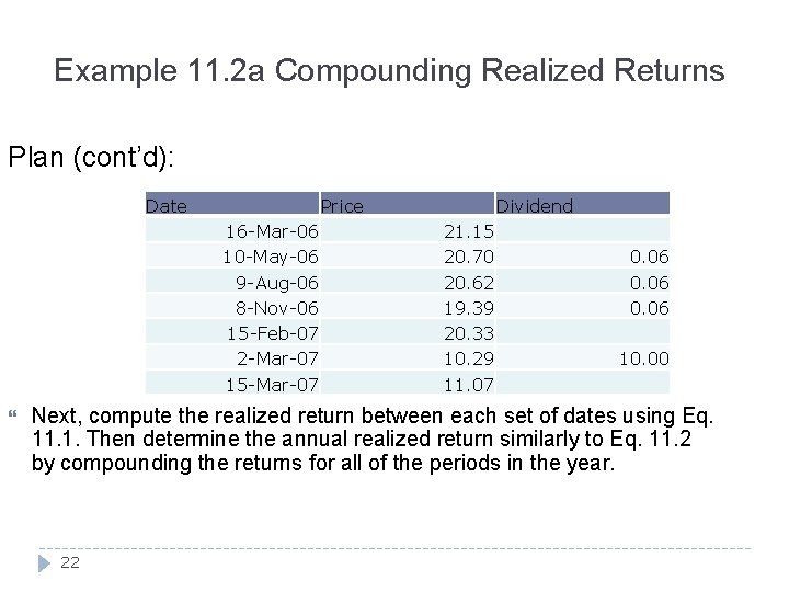
Example 11. 2 a Compounding Realized Returns Plan (cont’d): Date Price 16 -Mar-06 10 -May-06 9 -Aug-06 8 -Nov-06 15 -Feb-07 2 -Mar-07 15 -Mar-07 Dividend 21. 15 20. 70 20. 62 19. 39 20. 33 10. 29 11. 07 0. 06 10. 00 Next, compute the realized return between each set of dates using Eq. 11. 1. Then determine the annual realized return similarly to Eq. 11. 2 by compounding the returns for all of the periods in the year. 22

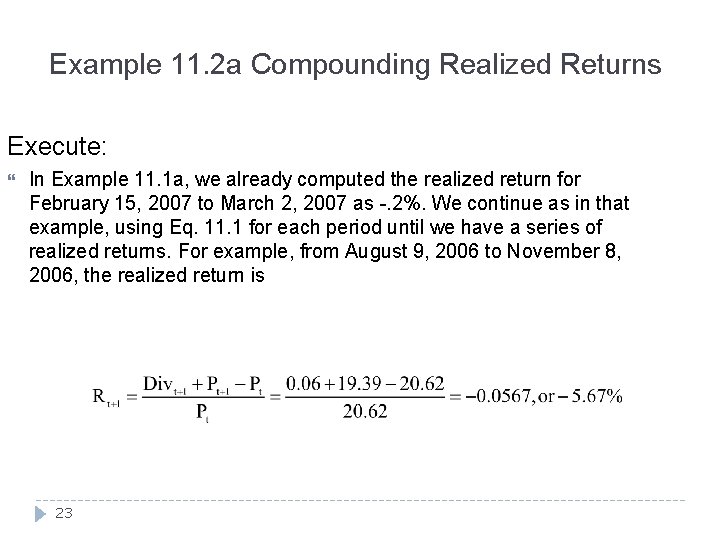
Example 11. 2 a Compounding Realized Returns Execute: In Example 11. 1 a, we already computed the realized return for February 15, 2007 to March 2, 2007 as -. 2%. We continue as in that example, using Eq. 11. 1 for each period until we have a series of realized returns. For example, from August 9, 2006 to November 8, 2006, the realized return is 23

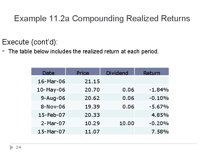
Example 11. 2 a Compounding Realized Returns Execute (cont’d): The table below includes the realized return at each period. Date 24 Price Dividend Return 16 -Mar-06 21. 15 10 -May-06 20. 70 0. 06 -1. 84% 9 -Aug-06 20. 62 0. 06 -0. 10% 8 -Nov-06 19. 39 0. 06 -5. 67% 15 -Feb-07 20. 33 2 -Mar-07 10. 29 15 -Mar-07 11. 07 4. 85% 10. 00 -0. 20% 7. 58%

Example 11. 2 a Compounding Realized Returns Execute (cont’d): We then determine the one-year return by compounding. 25

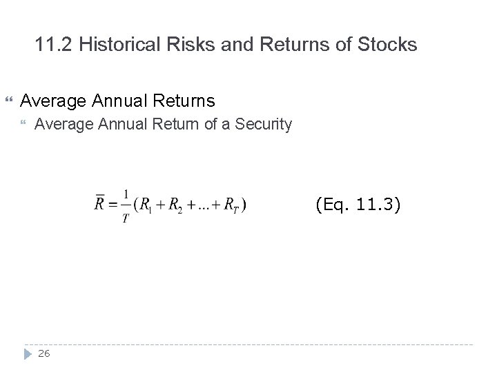
11. 2 Historical Risks and Returns of Stocks Average Annual Return of a Security (Eq. 11. 3) 26

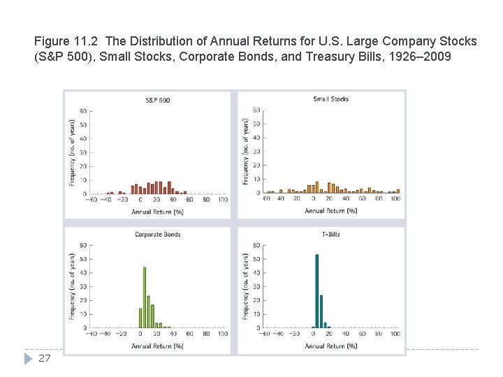
Figure 11. 2 The Distribution of Annual Returns for U. S. Large Company Stocks (S&P 500), Small Stocks, Corporate Bonds, and Treasury Bills, 1926– 2009 27

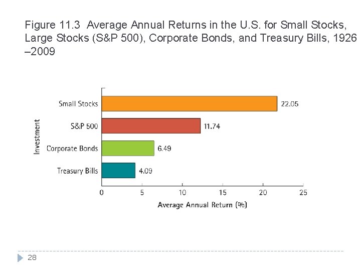
Figure 11. 3 Average Annual Returns in the U. S. for Small Stocks, Large Stocks (S&P 500), Corporate Bonds, and Treasury Bills, 1926 – 2009 28

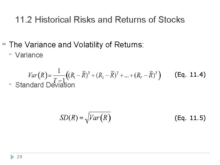
11. 2 Historical Risks and Returns of Stocks The Variance and Volatility of Returns: Variance (Eq. 11. 4) Standard Deviation (Eq. 11. 5) 29

Example 11. 3 Computing Historical Volatility Problem: Using the data from Table 11. 1, what is the standard deviation of the S&P 500’s returns for the years 2005 -2009? 30

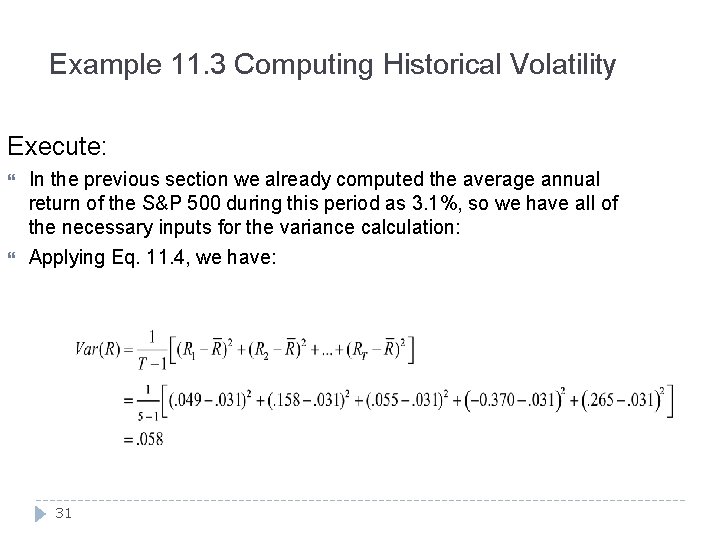
Example 11. 3 Computing Historical Volatility Execute: In the previous section we already computed the average annual return of the S&P 500 during this period as 3. 1%, so we have all of the necessary inputs for the variance calculation: Applying Eq. 11. 4, we have: 31

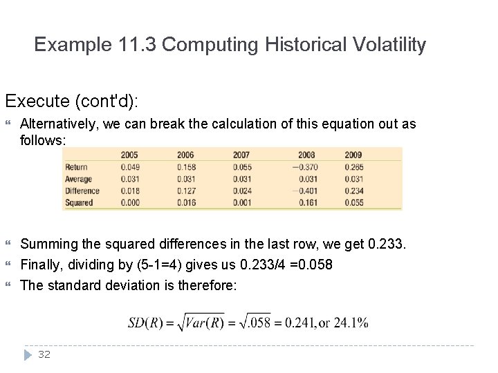
Example 11. 3 Computing Historical Volatility Execute (cont'd): Alternatively, we can break the calculation of this equation out as follows: Summing the squared differences in the last row, we get 0. 233. Finally, dividing by (5 -1=4) gives us 0. 233/4 =0. 058 The standard deviation is therefore: 32

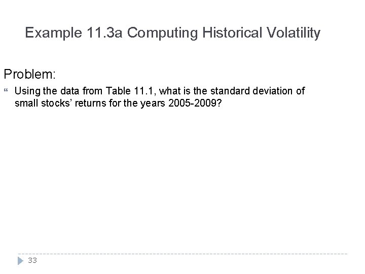
Example 11. 3 a Computing Historical Volatility Problem: Using the data from Table 11. 1, what is the standard deviation of small stocks’ returns for the years 2005 -2009? 33

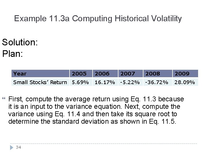
Example 11. 3 a Computing Historical Volatility Solution: Plan: Year 2005 Small Stocks’ Return 5. 69% 2006 2007 16. 17% -5. 22% 2008 2009 -36. 72% 28. 09% First, compute the average return using Eq. 11. 3 because it is an input to the variance equation. Next, compute the variance using Eq. 11. 4 and then take its square root to determine the standard deviation as shown in Eq. 11. 5. 34

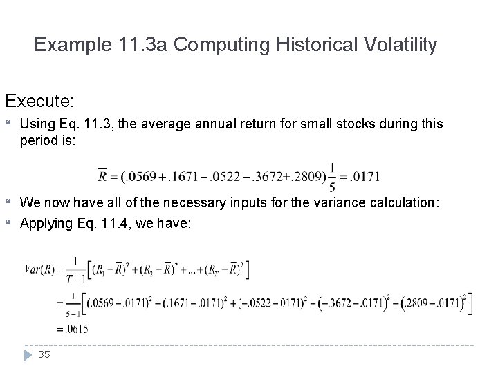
Example 11. 3 a Computing Historical Volatility Execute: Using Eq. 11. 3, the average annual return for small stocks during this period is: We now have all of the necessary inputs for the variance calculation: Applying Eq. 11. 4, we have: 35

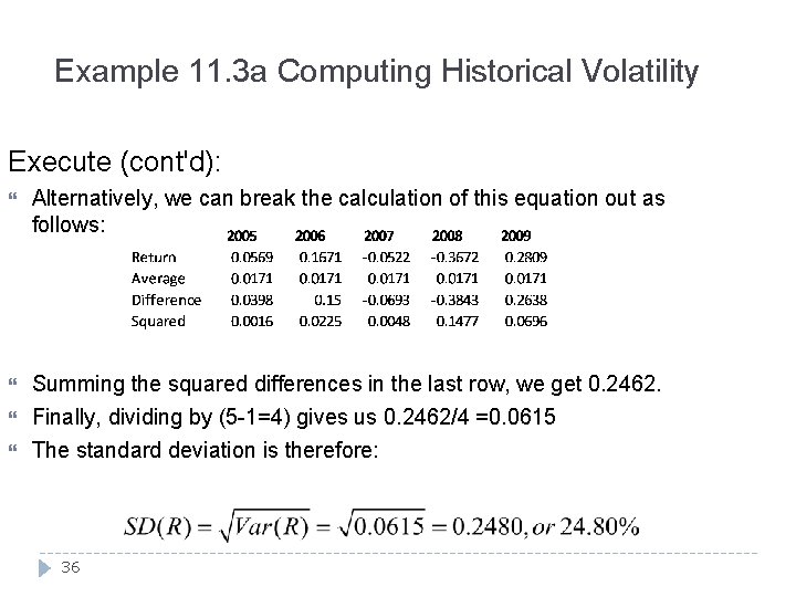
Example 11. 3 a Computing Historical Volatility Execute (cont'd): Alternatively, we can break the calculation of this equation out as follows: Summing the squared differences in the last row, we get 0. 2462. Finally, dividing by (5 -1=4) gives us 0. 2462/4 =0. 0615 The standard deviation is therefore: 36

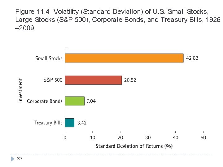
Figure 11. 4 Volatility (Standard Deviation) of U. S. Small Stocks, Large Stocks (S&P 500), Corporate Bonds, and Treasury Bills, 1926 – 2009 37

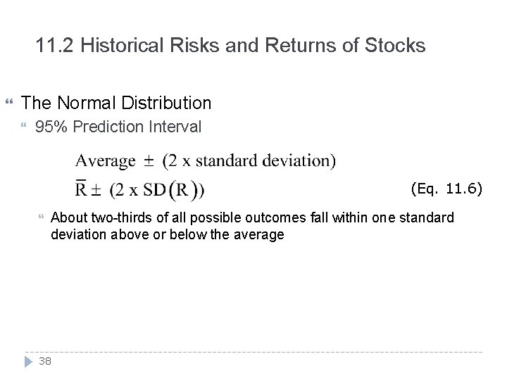
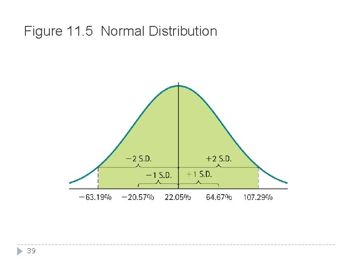
11. 2 Historical Risks and Returns of Stocks The Normal Distribution 95% Prediction Interval (Eq. 11. 6) About two-thirds of all possible outcomes fall within one standard deviation above or below the average 38

Figure 11. 5 Normal Distribution 39

Example 11. 4 Confidence Intervals Problem: In Example 11. 3 we found the average return for the S&P 500 from 2005 -2009 to be 3. 1% with a standard deviation of 24. 1%. What is a 95% confidence interval for 2010’s return? 40

Example 11. 4 Confidence Intervals Solution: Plan: We can use Eq. 11. 6 to compute the confidence interval. 41

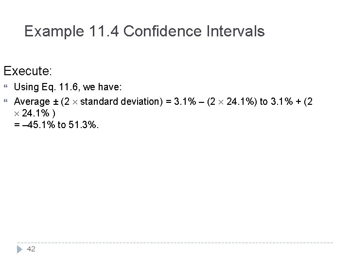
Example 11. 4 Confidence Intervals Execute: Using Eq. 11. 6, we have: Average ± (2 standard deviation) = 3. 1% – (2 24. 1%) to 3. 1% + (2 24. 1% ) = – 45. 1% to 51. 3%. 42

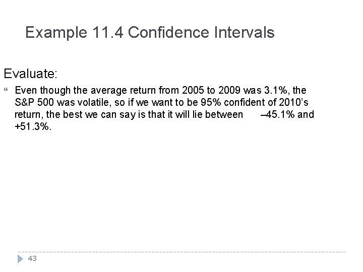
Example 11. 4 Confidence Intervals Evaluate: Even though the average return from 2005 to 2009 was 3. 1%, the S&P 500 was volatile, so if we want to be 95% confident of 2010’s return, the best we can say is that it will lie between – 45. 1% and +51. 3%. 43

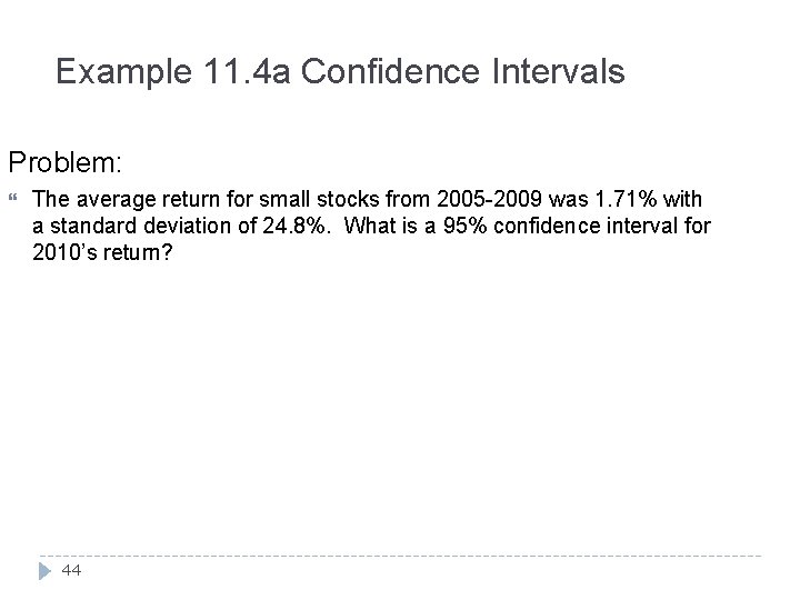
Example 11. 4 a Confidence Intervals Problem: The average return for small stocks from 2005 -2009 was 1. 71% with a standard deviation of 24. 8%. What is a 95% confidence interval for 2010’s return? 44

Example 11. 4 a Confidence Intervals Solution: Plan: We can use Eq. 11. 6 to calculate the confidence interval. 45

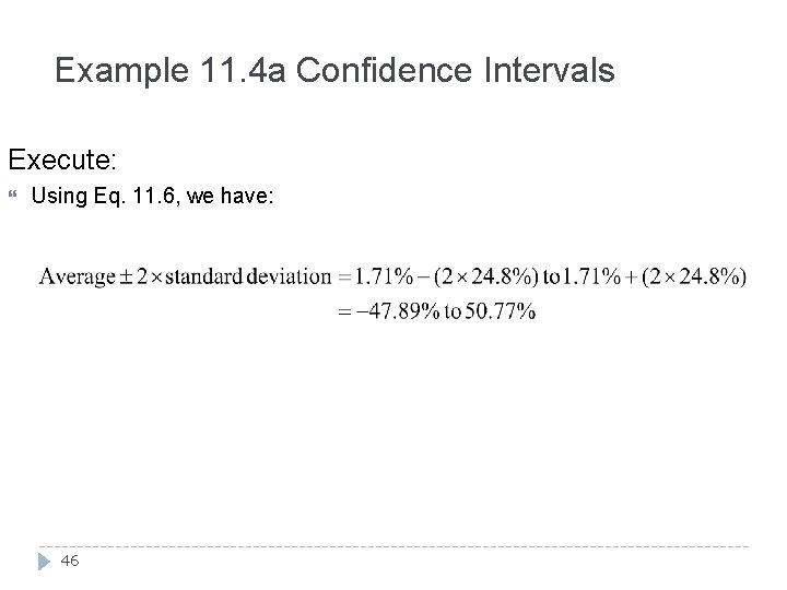
Example 11. 4 a Confidence Intervals Execute: Using Eq. 11. 6, we have: 46

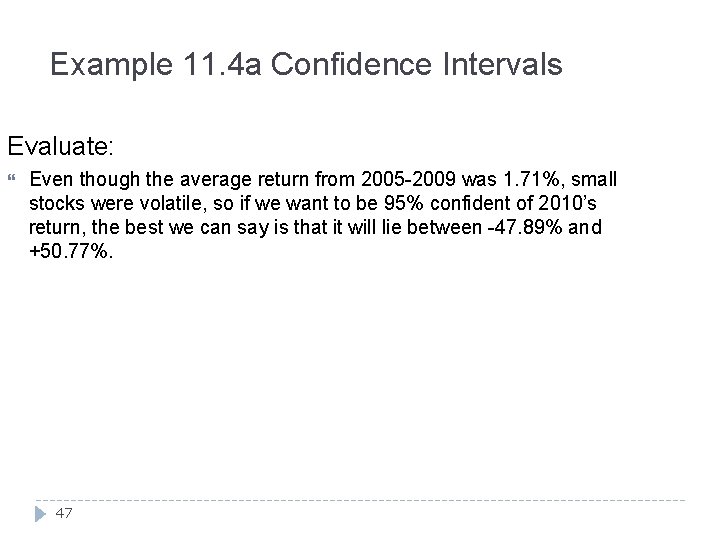
Example 11. 4 a Confidence Intervals Evaluate: Even though the average return from 2005 -2009 was 1. 71%, small stocks were volatile, so if we want to be 95% confident of 2010’s return, the best we can say is that it will lie between -47. 89% and +50. 77%. 47

Example 11. 4 b Confidence Intervals Problem: The average return for corporate bonds from 2005 -2009 was 6. 49% with a standard deviation of 7. 04%. What is a 95% confidence interval for 2010’s return? 48

Example 11. 4 b Confidence Intervals Solution: Plan: We can use Eq. 11. 6 to calculate the confidence interval. 49

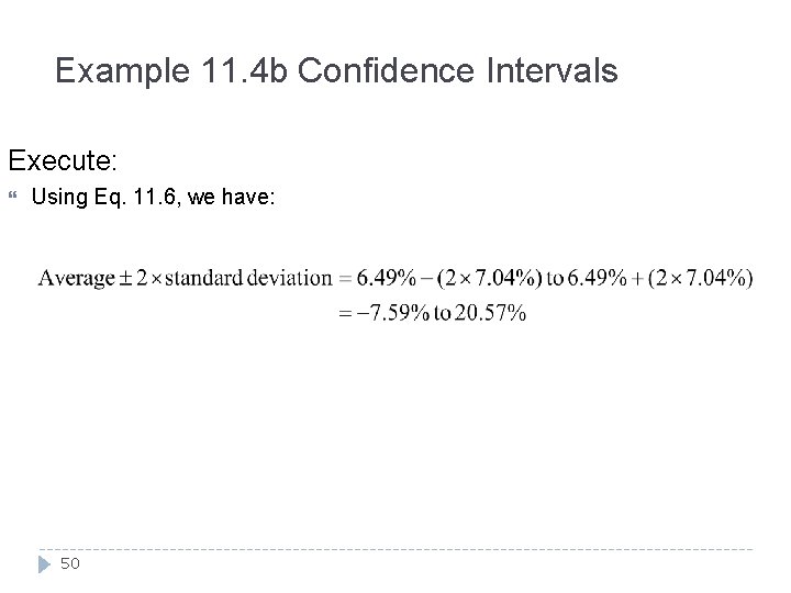
Example 11. 4 b Confidence Intervals Execute: Using Eq. 11. 6, we have: 50

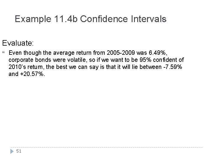
Example 11. 4 b Confidence Intervals Evaluate: Even though the average return from 2005 -2009 was 6. 49%, corporate bonds were volatile, so if we want to be 95% confident of 2010’s return, the best we can say is that it will lie between -7. 59% and +20. 57%. 51

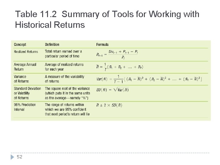
Table 11. 2 Summary of Tools for Working with Historical Returns 52

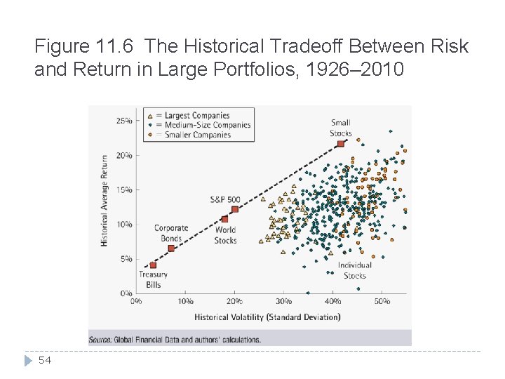
11. 3 Historical Tradeoff between Risk and Return The Returns of Large Portfolios Investments with higher volatility, as measured by standard deviation, tend to have higher average returns 53

Figure 11. 6 The Historical Tradeoff Between Risk and Return in Large Portfolios, 1926– 2010 54

11. 3 Historical Tradeoff between Risk and Return The Returns of Individual Stocks Larger stocks have lower volatility overall Even the largest stocks are typically more volatile than a portfolio of large stocks The standard deviation of an individual security doesn’t explain the size of its average return All individual stocks have lower returns and/or higher risk than the portfolios in Figure 11. 6 55

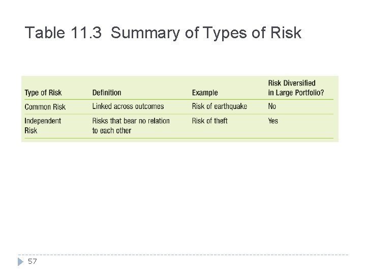
11. 4 Common Versus Independent Risk Types of Risk Common Risk Independent Risk Diversification 56

Table 11. 3 Summary of Types of Risk 57

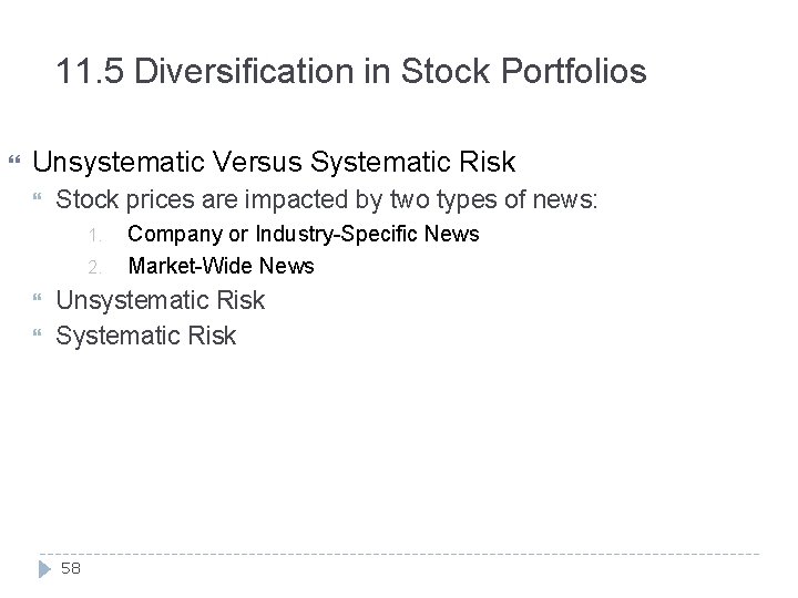
11. 5 Diversification in Stock Portfolios Unsystematic Versus Systematic Risk Stock prices are impacted by two types of news: 1. 2. Company or Industry-Specific News Market-Wide News Unsystematic Risk Systematic Risk 58

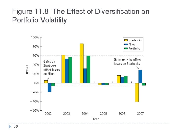
Figure 11. 8 The Effect of Diversification on Portfolio Volatility 59

11. 5 Diversification in Stock Portfolios Diversifiable Risk and the Risk Premium The risk premium for diversifiable risk is zero Investors are not compensated for holding unsystematic risk 60

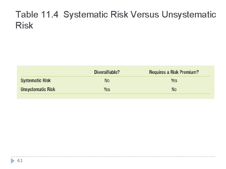
Table 11. 4 Systematic Risk Versus Unsystematic Risk 61

11. 5 Diversification in Stock Portfolios The Importance of Systematic Risk The risk premium of a security is determined by its systematic risk and does not depend on its diversifiable risk 62

11. 5 Diversification in Stock Portfolios The Importance of Systematic Risk There is no relationship between volatility and average returns for individual securities 63

References 64

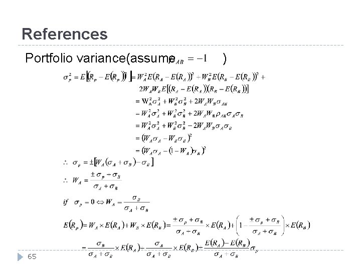
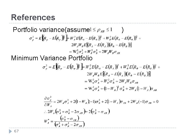
References Portfolio variance(assume ) 65

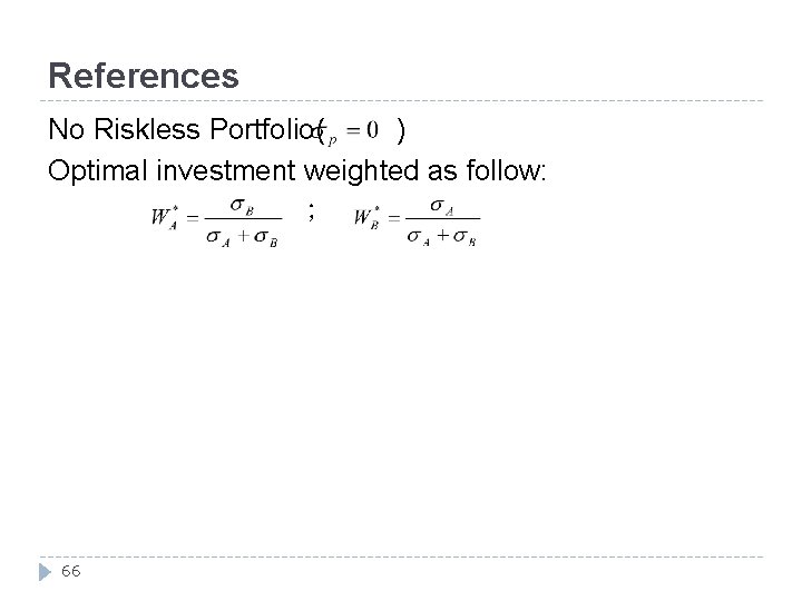
References No Riskless Portfolio( ) Optimal investment weighted as follow: ； 66

References Portfolio variance(assume ) Minimum Variance Portfolio 67

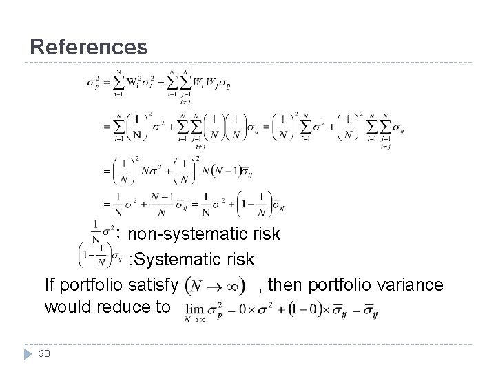
References ：non-systematic risk : Systematic risk If portfolio satisfy , then portfolio variance would reduce to 68