CHAPTER 8 Risk and Rates of Return n

CHAPTER 8 Risk and Rates of Return n Stand-alone risk Portfolio risk Risk & return: CAPM / SML 8 -1

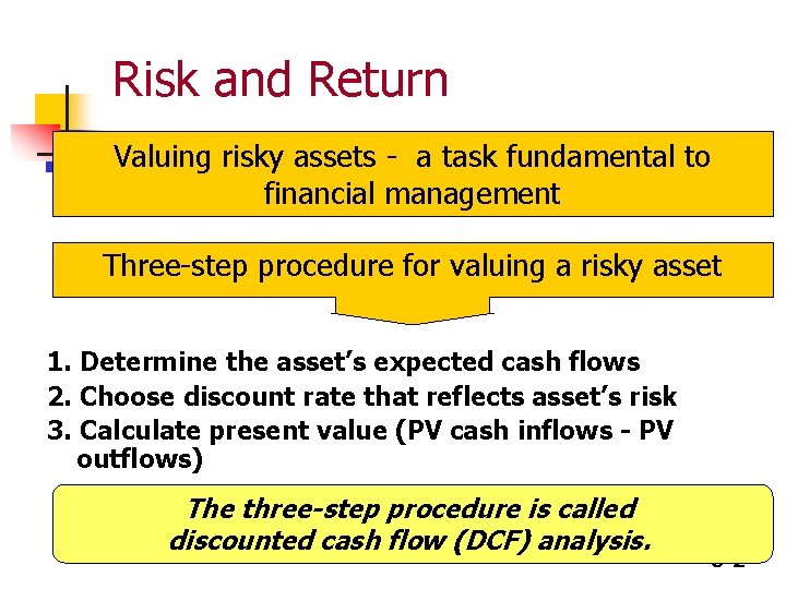
Risk and Return Valuing risky assets - a task fundamental to financial management Three-step procedure for valuing a risky asset 1. Determine the asset’s expected cash flows 2. Choose discount rate that reflects asset’s risk 3. Calculate present value (PV cash inflows - PV outflows) The three-step procedure is called discounted cash flow (DCF) analysis. 8 -2

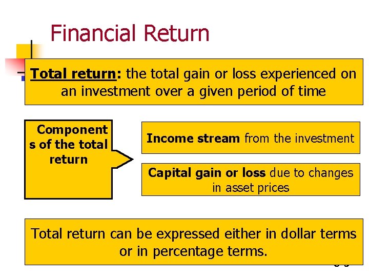
Financial Return Total return: the total gain or loss experienced on an investment over a given period of time Component s of the total return Income stream from the investment Capital gain or loss due to changes in asset prices Total return can be expressed either in dollar terms or in percentage terms. 8 -3

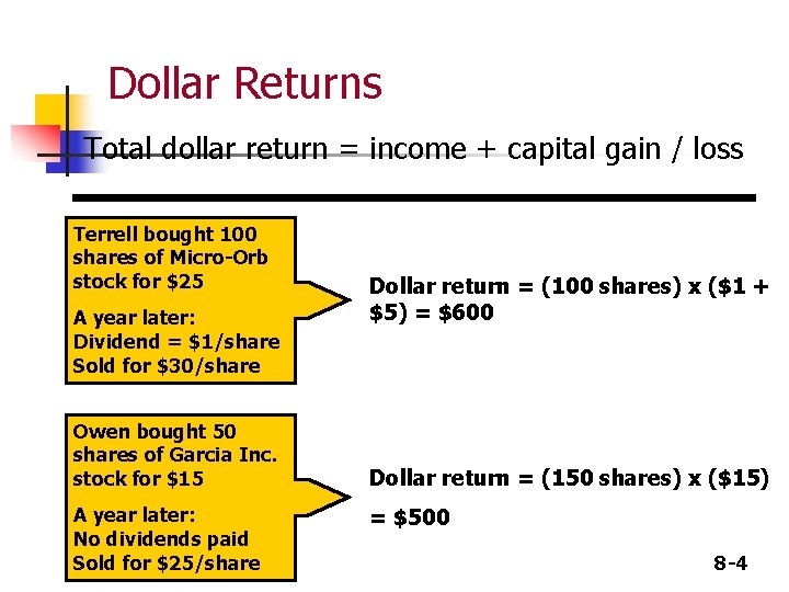
Dollar Returns Total dollar return = income + capital gain / loss Terrell bought 100 shares of Micro-Orb stock for $25 A year later: Dividend = $1/share Sold for $30/share Owen bought 50 shares of Garcia Inc. stock for $15 A year later: No dividends paid Sold for $25/share Dollar return = (100 shares) x ($1 + $5) = $600 Dollar return = (150 shares) x ($15) = $500 8 -4

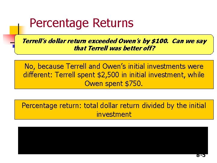
Percentage Returns Terrell’s dollar return exceeded Owen’s by $100. Can we say that Terrell was better off? No, because Terrell and Owen’s initial investments were different: Terrell spent $2, 500 in initial investment, while Owen spent $750. Percentage return: total dollar return divided by the initial investment 8 -5

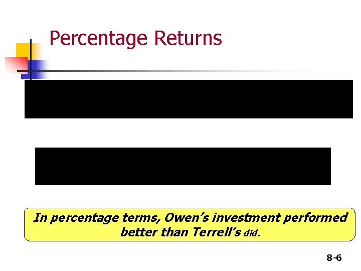
Percentage Returns In percentage terms, Owen’s investment performed better than Terrell’s did. 8 -6

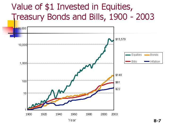
Value of $1 Invested in Equities, Treasury Bonds and Bills, 1900 - 2003 100, 000 $15, 579 10, 000 1, 000 Equities Bonds Bills Inflation $148 100 $61 $22 10 1 1900 1920 1940 1960 Year 1980 2003 8 -7

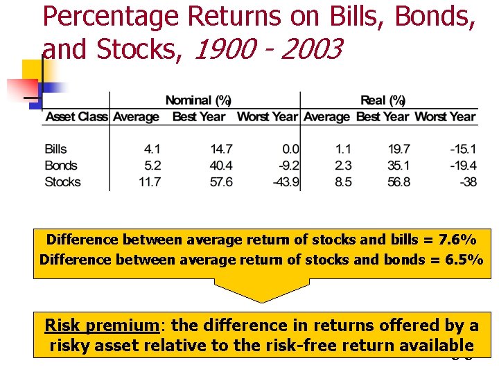
Percentage Returns on Bills, Bonds, and Stocks, 1900 - 2003 Difference between average return of stocks and bills = 7. 6% Difference between average return of stocks and bonds = 6. 5% Risk premium: the difference in returns offered by a risky asset relative to the risk-free return available 8 -8

Video: Dimson Smart Finance 8 -9

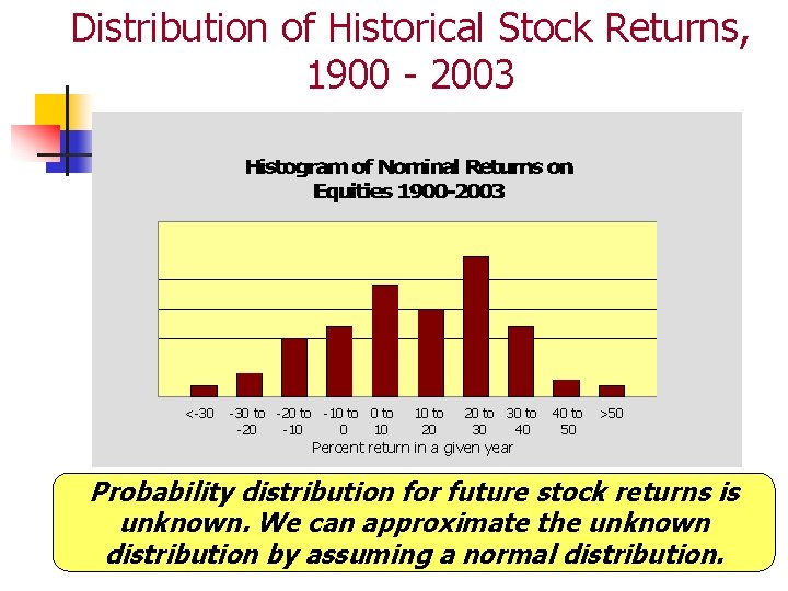
Distribution of Historical Stock Returns, 1900 - 2003 <-30 to -20 to -10 to -20 -10 0 10 10 to 20 20 to 30 40 40 to 50 >50 Percent return in a given year Probability distribution for future stock returns is unknown. We can approximate the unknown distribution by assuming a normal distribution. 8 -10

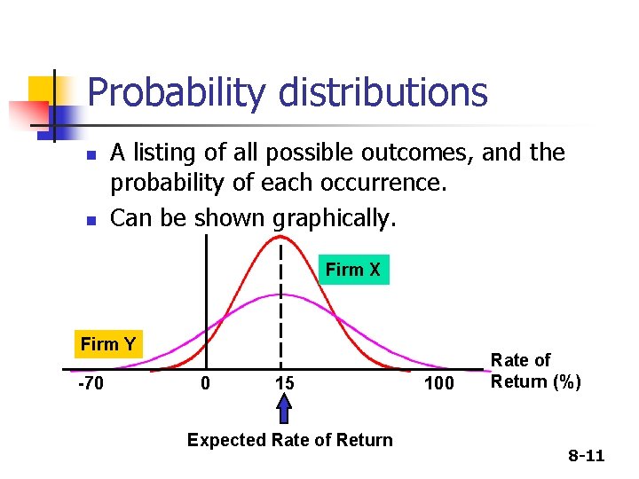
Probability distributions n n A listing of all possible outcomes, and the probability of each occurrence. Can be shown graphically. Firm X Firm Y -70 0 15 Expected Rate of Return 100 Rate of Return (%) 8 -11

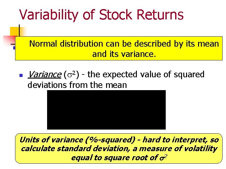
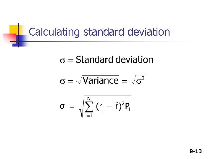
Variability of Stock Returns Normal distribution can be described by its mean and its variance. n Variance ( 2) - the expected value of squared deviations from the mean Units of variance (%-squared) - hard to interpret, so calculate standard deviation, a measure of volatility equal to square root of 2 8 -12

Calculating standard deviation 8 -13

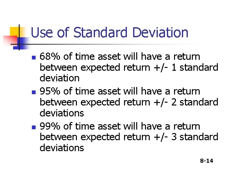
Use of Standard Deviation n 68% of time asset will have a return between expected return +/- 1 standard deviation 95% of time asset will have a return between expected return +/- 2 standard deviations 99% of time asset will have a return between expected return +/- 3 standard deviations 8 -14

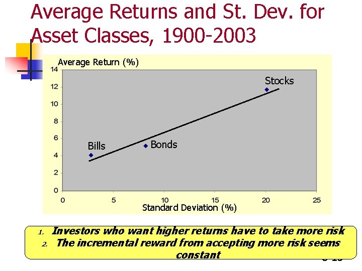
Average Returns and St. Dev. for Asset Classes, 1900 -2003 Average Return (%) Stocks Bills Bonds Standard Deviation (%) 1. 2. Investors who want higher returns have to take more risk The incremental reward from accepting more risk seems constant 8 -15

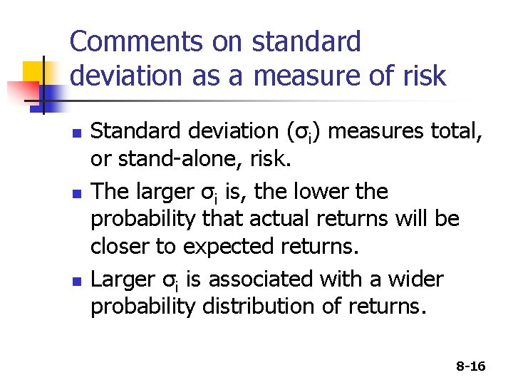
Comments on standard deviation as a measure of risk n n n Standard deviation (σi) measures total, or stand-alone, risk. The larger σi is, the lower the probability that actual returns will be closer to expected returns. Larger σi is associated with a wider probability distribution of returns. 8 -16

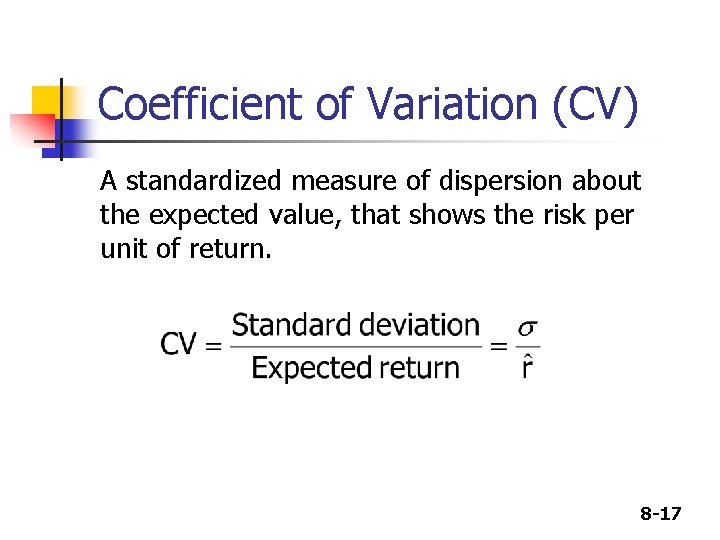
Coefficient of Variation (CV) A standardized measure of dispersion about the expected value, that shows the risk per unit of return. 8 -17

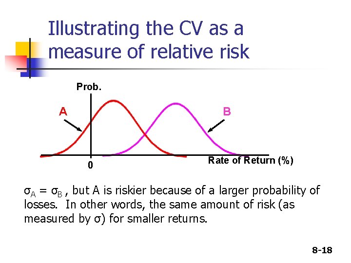
Illustrating the CV as a measure of relative risk Prob. A B 0 Rate of Return (%) σA = σB , but A is riskier because of a larger probability of losses. In other words, the same amount of risk (as measured by σ) for smaller returns. 8 -18

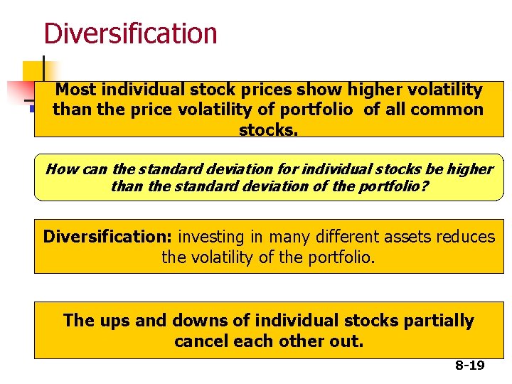
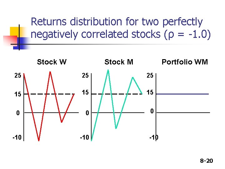
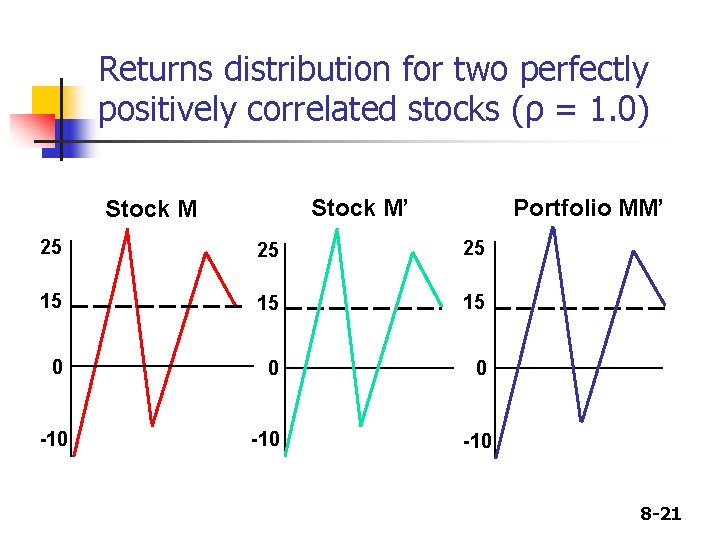
Diversification Most individual stock prices show higher volatility than the price volatility of portfolio of all common stocks. How can the standard deviation for individual stocks be higher than the standard deviation of the portfolio? Diversification: investing in many different assets reduces the volatility of the portfolio. The ups and downs of individual stocks partially cancel each other out. 8 -19

Returns distribution for two perfectly negatively correlated stocks (ρ = -1. 0) Stock W Stock M Portfolio WM 25 25 25 15 15 15 0 0 0 -10 -10 8 -20

Returns distribution for two perfectly positively correlated stocks (ρ = 1. 0) Stock M’ Stock M Portfolio MM’ 25 25 25 15 15 15 0 0 0 -10 -10 8 -21

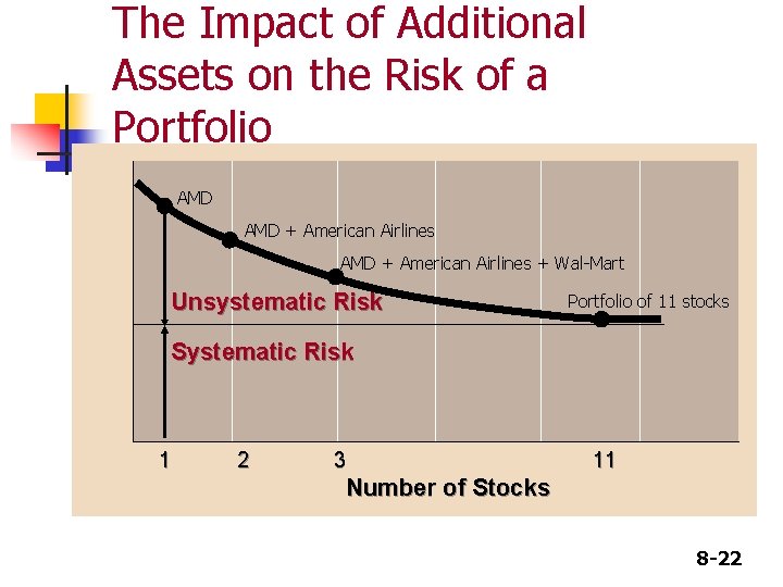
Portfolio Standard Deviation The Impact of Additional Assets on the Risk of a Portfolio AMD + American Airlines + Wal-Mart Unsystematic Risk Portfolio of 11 stocks Systematic Risk 1 2 3 11 Number of Stocks 8 -22

Systematic and Unsystematic Risk Diversification reduces portfolio volatility, but only up to a point. Portfolio of all stocks still has a volatility of 21%. Systematic risk: the volatility of the portfolio that cannot be eliminated through diversification. Unsystematic risk: the proportion of risk of individual assets that can be eliminated through diversification What really matters is systematic risk…. how a group of assets move together. 8 -23

Systematic and Unsystematic Risk Anheuser Busch stock had higher average returns than Archer-Daniels-Midland stock, with smaller volatility. American Airlines had much smaller average returns than Wal-Mart, with similar volatility. The tradeoff between standard deviation and average returns that holds for asset classes does not hold for individual stocks. Standard deviation contains both systematic and unsystematic risk. Because investors can eliminate unsystematic risk through diversification, market rewards only 8 -24 systematic risk.

Video: Sharpe(in 7) Smart Finance 8 -25

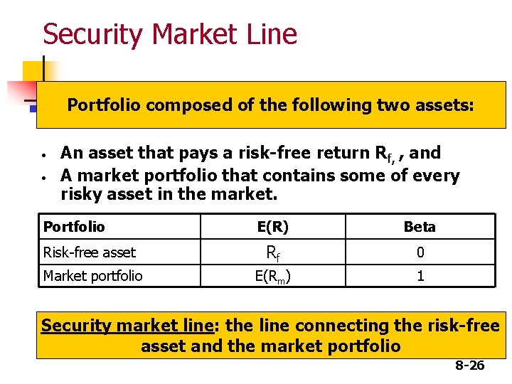
Security Market Line Portfolio composed of the following two assets: • • An asset that pays a risk-free return Rf, , and A market portfolio that contains some of every risky asset in the market. Portfolio E(R) Beta Risk-free asset Rf 0 Market portfolio E(Rm) 1 Security market line: the line connecting the risk-free asset and the market portfolio 8 -26

Beta n n Measures a stock’s market risk, and shows a stock’s volatility relative to the market. Indicates how risky a stock is if the stock is held in a well-diversified portfolio. 8 -27

Comments on beta n n If beta = 1. 0, the security is just as risky as the average stock. If beta > 1. 0, the security is riskier than average. If beta < 1. 0, the security is less risky than average. Most stocks have betas in the range of 0. 5 to 1. 5. 8 -28

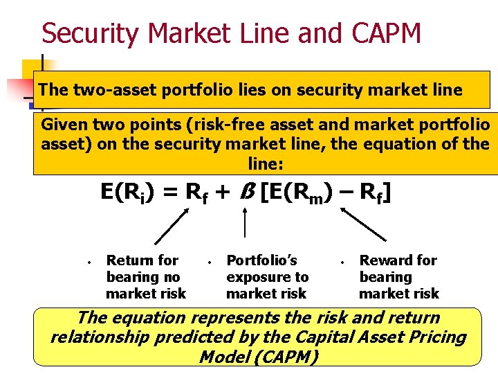
Security Market Line and CAPM The two-asset portfolio lies on security market line Given two points (risk-free asset and market portfolio asset) on the security market line, the equation of the line: E(Ri) = Rf + ß [E(Rm) – Rf] • Return for bearing no market risk • Portfolio’s exposure to market risk • Reward for bearing market risk The equation represents the risk and return relationship predicted by the Capital Asset Pricing 8 -29 Model (CAPM)

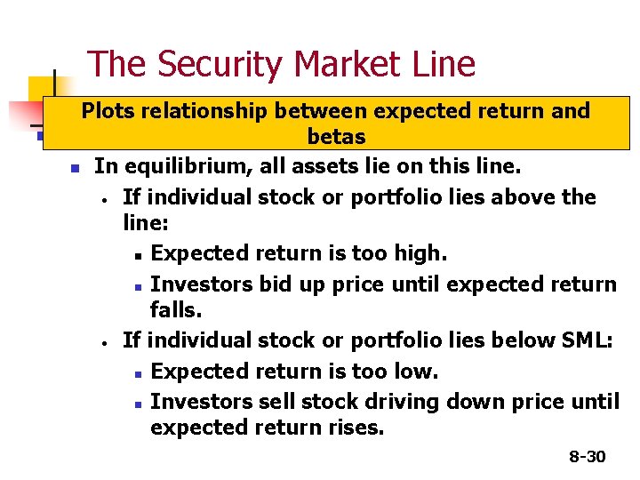
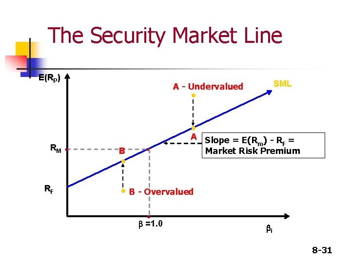
The Security Market Line Plots relationship between expected return and betas n In equilibrium, all assets lie on this line. • If individual stock or portfolio lies above the line: n Expected return is too high. n Investors bid up price until expected return falls. • If individual stock or portfolio lies below SML: n Expected return is too low. n Investors sell stock driving down price until expected return rises. 8 -30

The Security Market Line E(RP) SML A - Undervalued • • RM RF • B • • A Slope = E(R ) - R = m F Market Risk Premium • B - Overvalued • =1. 0 i 8 -31