Chapter 8 Risk and Return Copyright 2010 Pearson

Chapter 8 • Risk and Return Copyright © 2010 Pearson Prentice Hall. All rights reserved.

Learning Objectives 1. Calculate profits and returns on an investment and convert holding period returns to annual returns. 2. Define risk and explain how uncertainty relates to risk. 3. Appreciate the historical returns of various investment choices. 4. Calculate standard deviations and variances with historical data. 5. Calculate expected returns and variances with conditional returns and probabilities. Copyright © 2010 Pearson Prentice Hall. All rights reserved. 8 -2

Learning Objectives 6. Interpret the trade-off between risk and return. 7. Understand when and why diversification works at minimizing risk, and understand the difference between systematic and unsystematic risk. 8. Explain beta as a measure of risk in a well-diversified portfolio. 9. Illustrate how the security market line and the capital asset pricing model represent the twoparameter world of risk and return. Copyright © 2010 Pearson Prentice Hall. All rights reserved. 8 -3

8. 1 Returns • All investors want to maximize return and minimize risk. This the risk-and-return trade-off, or the “ability-to-sleep-at-night test. ” • Performance analysis of an investment requires investors to measure returns over time. • Because return and risk are intricately related, the measurement of return helps in the understanding of investment risk. Copyright © 2010 Pearson Prentice Hall. All rights reserved. 8 -4

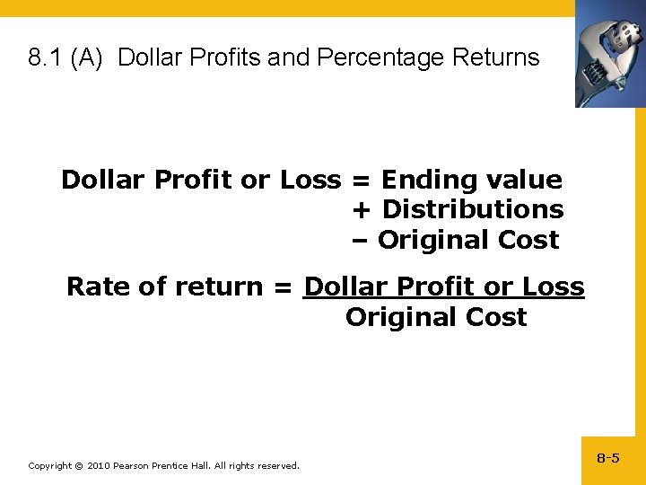
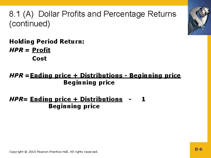
8. 1 (A) Dollar Profits and Percentage Returns Dollar Profit or Loss = Ending value + Distributions – Original Cost Rate of return = Dollar Profit or Loss Original Cost Copyright © 2010 Pearson Prentice Hall. All rights reserved. 8 -5

8. 1 (A) Dollar Profits and Percentage Returns (continued) Holding Period Return: HPR = Profit Cost HPR =Ending price + Distributions - Beginning price HPR= Ending price + Distributions - 1 Beginning price Copyright © 2010 Pearson Prentice Hall. All rights reserved. 8 -6

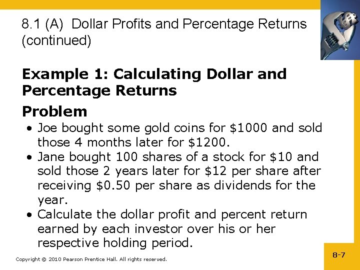
8. 1 (A) Dollar Profits and Percentage Returns (continued) Example 1: Calculating Dollar and Percentage Returns Problem • Joe bought some gold coins for $1000 and sold those 4 months later for $1200. • Jane bought 100 shares of a stock for $10 and sold those 2 years later for $12 per share after receiving $0. 50 per share as dividends for the year. • Calculate the dollar profit and percent return earned by each investor over his or her respective holding period. Copyright © 2010 Pearson Prentice Hall. All rights reserved. 8 -7

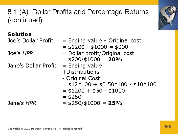
8. 1 (A) Dollar Profits and Percentage Returns (continued) Solution Joe’s Dollar Profit Joe’s HPR Jane’s Dollar Profit Jane’s HPR = Ending value – Original cost = $1200 - $1000 = $200 = Dollar profit/Original cost = $200/$1000 = 20% = Ending value +Distributions - Original Cost = $12*100 + $0. 50*100 - $10*100 = $1200 + $50 - $1000 = $250/$1000 = 25% Copyright © 2010 Pearson Prentice Hall. All rights reserved. 8 -8

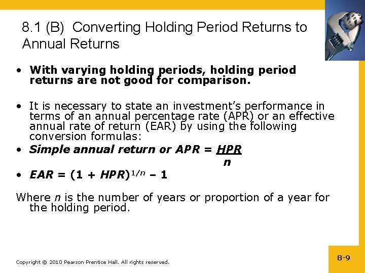
8. 1 (B) Converting Holding Period Returns to Annual Returns • With varying holding periods, holding period returns are not good for comparison. • It is necessary to state an investment’s performance in terms of an annual percentage rate (APR) or an effective annual rate of return (EAR) by using the following conversion formulas: • Simple annual return or APR = HPR n • EAR = (1 + HPR)1/n – 1 Where n is the number of years or proportion of a year for the holding period. Copyright © 2010 Pearson Prentice Hall. All rights reserved. 8 -9

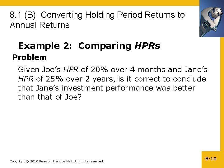
8. 1 (B) Converting Holding Period Returns to Annual Returns Example 2: Comparing HPRs Problem Given Joe’s HPR of 20% over 4 months and Jane’s HPR of 25% over 2 years, is it correct to conclude that Jane’s investment performance was better than that of Joe? Copyright © 2010 Pearson Prentice Hall. All rights reserved. 8 -10

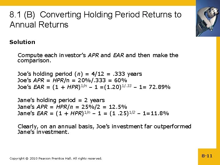
8. 1 (B) Converting Holding Period Returns to Annual Returns Solution Compute each investor’s APR and EAR and then make the comparison. Joe’s holding period (n) = 4/12 =. 333 years Joe’s APR = HPR/n = 20%/. 333 = 60% Joe’s EAR = (1 + HPR)1/n – 1 =(1. 20)1/. 33 – 1= 72. 89% Jane’s holding period = 2 years Jane’s APR = HPR/n = 25%/2 = 12. 5% Jane’s EAR = (1 + HPR)1/n – 1 = (1. 25)1/2 – 1=11. 8% Clearly, on an annual basis, Joe’s investment far outperformed Jane’s investment. Copyright © 2010 Pearson Prentice Hall. All rights reserved. 8 -11

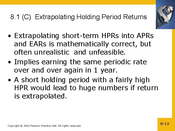
8. 1 (C) Extrapolating Holding Period Returns • Extrapolating short-term HPRs into APRs and EARs is mathematically correct, but often unrealistic and unfeasible. • Implies earning the same periodic rate over and over again in 1 year. • A short holding period with a fairly high HPR would lead to huge numbers if return is extrapolated. Copyright © 2010 Pearson Prentice Hall. All rights reserved. 8 -12

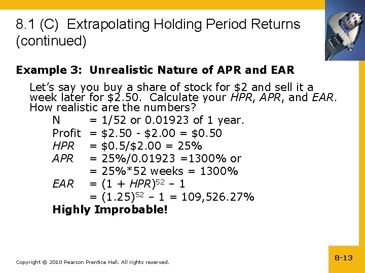
8. 1 (C) Extrapolating Holding Period Returns (continued) Example 3: Unrealistic Nature of APR and EAR Let’s say you buy a share of stock for $2 and sell it a week later for $2. 50. Calculate your HPR, APR, and EAR. How realistic are the numbers? N = 1/52 or 0. 01923 of 1 year. Profit = $2. 50 - $2. 00 = $0. 50 HPR = $0. 5/$2. 00 = 25% APR = 25%/0. 01923 =1300% or = 25%*52 weeks = 1300% EAR = (1 + HPR)52 – 1 = (1. 25)52 – 1 = 109, 526. 27% Highly Improbable! Copyright © 2010 Pearson Prentice Hall. All rights reserved. 8 -13

8. 2 Risk (Certainty and Uncertainty) • Future performance of most investments is uncertain. • Risky Potential for loss exists • Risk can be defined as a measure of the uncertainty in a set of potential outcomes for an event in which there is a chance of some loss. • It is important to measure and analyze the risk potential of an investment so as to make an informed decision. Copyright © 2010 Pearson Prentice Hall. All rights reserved. 8 -14

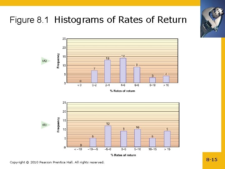
Figure 8. 1 Histograms of Rates of Return Copyright © 2010 Pearson Prentice Hall. All rights reserved. 8 -15

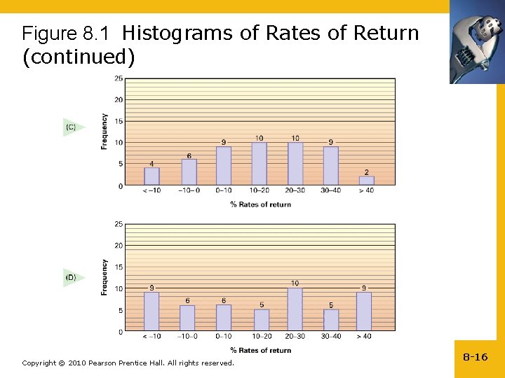
Figure 8. 1 Histograms of Rates of Return (continued) Copyright © 2010 Pearson Prentice Hall. All rights reserved. 8 -16

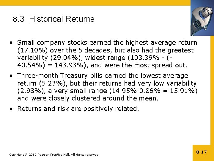
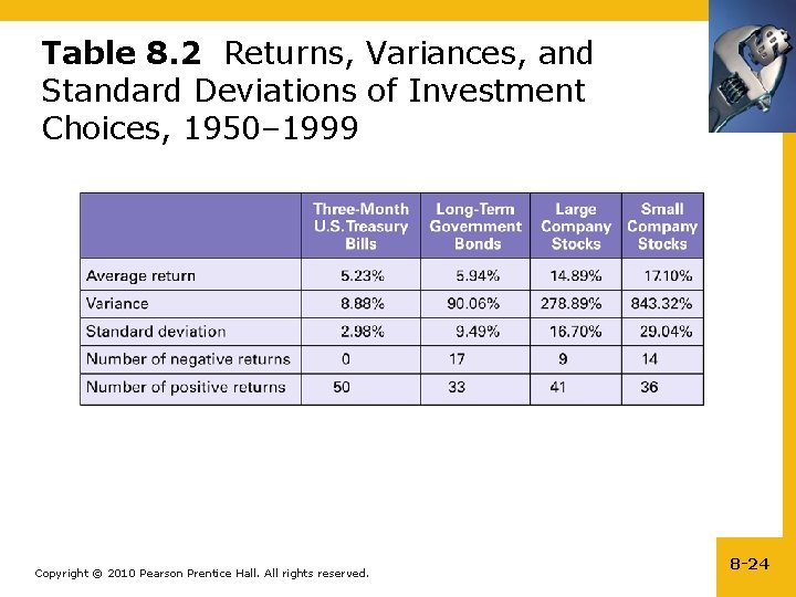
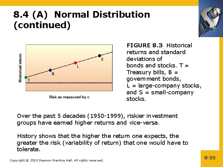
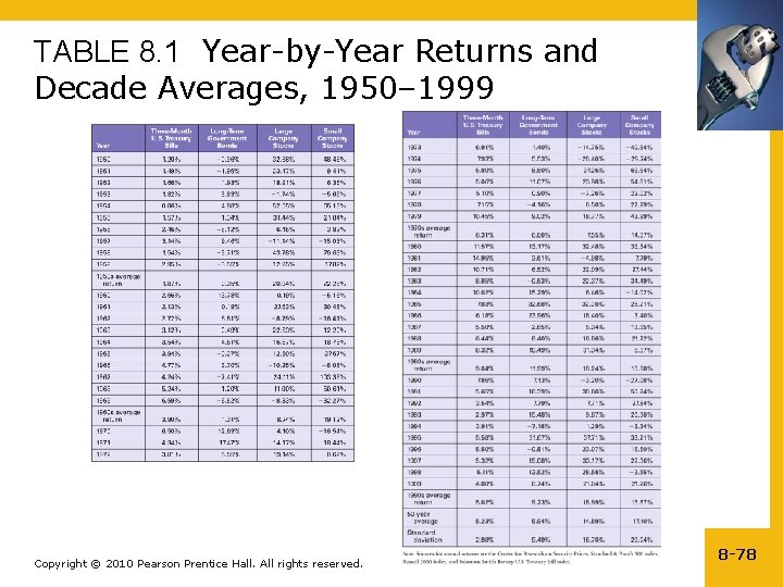
8. 3 Historical Returns • Small company stocks earned the highest average return (17. 10%) over the 5 decades, but also had the greatest variability (29. 04%), widest range (103. 39% - (40. 54%) = 143. 93%), and were the most spread out. • Three-month Treasury bills earned the lowest average return (5. 23%), but their returns had very low variability (2. 98%), a very small range (14. 95%-0. 86% = 15. 91%) and were closely clustered around the mean. • Returns and risk are positively related. Copyright © 2010 Pearson Prentice Hall. All rights reserved. 8 -17

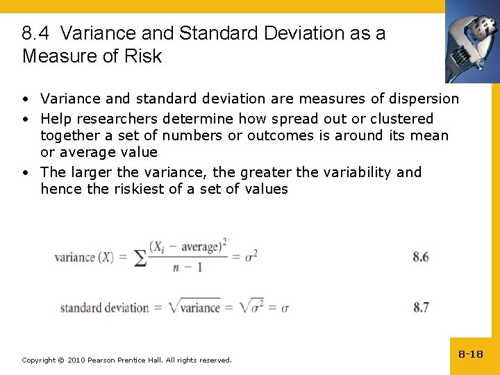
8. 4 Variance and Standard Deviation as a Measure of Risk • Variance and standard deviation are measures of dispersion • Help researchers determine how spread out or clustered together a set of numbers or outcomes is around its mean or average value • The larger the variance, the greater the variability and hence the riskiest of a set of values Copyright © 2010 Pearson Prentice Hall. All rights reserved. 8 -18

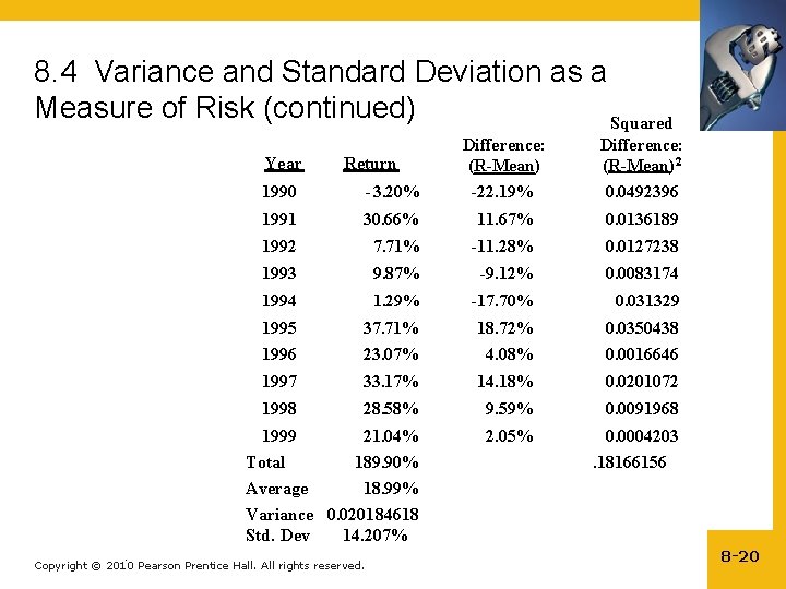
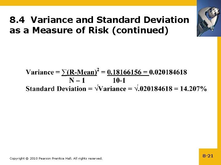
8. 4 Variance and Standard Deviation as a Measure of Risk (continued) Example 4: Calculating the Variance of Returns for Large-Company Stocks Problem Listed on the following slide are the annual returns associated with the large-company stock portfolio from 1990 - 1999. Calculate the variance and standard deviation of the returns. Copyright © 2010 Pearson Prentice Hall. All rights reserved. 8 -19

8. 4 Variance and Standard Deviation as a Measure of Risk (continued) Squared Difference: (R-Mean)2 1990 -3. 20% Difference: (R-Mean) -22. 19% 1991 30. 66% 11. 67% 0. 0136189 1992 7. 71% -11. 28% 0. 0127238 1993 9. 87% -9. 12% 0. 0083174 1994 1. 29% -17. 70% 0. 031329 1995 37. 71% 18. 72% 0. 0350438 1996 23. 07% 4. 08% 0. 0016646 1997 33. 17% 14. 18% 0. 0201072 1998 28. 58% 9. 59% 0. 0091968 1999 Total 21. 04% 189. 90% 2. 05% 0. 0004203. 18166156 Year Return 0. 0492396 Average 18. 99% Variance 0. 020184618 Std. Dev 14. 207%. Copyright © 2010 Pearson Prentice Hall. All rights reserved. 8 -20

8. 4 Variance and Standard Deviation as a Measure of Risk (continued) Copyright © 2010 Pearson Prentice Hall. All rights reserved. 8 -21

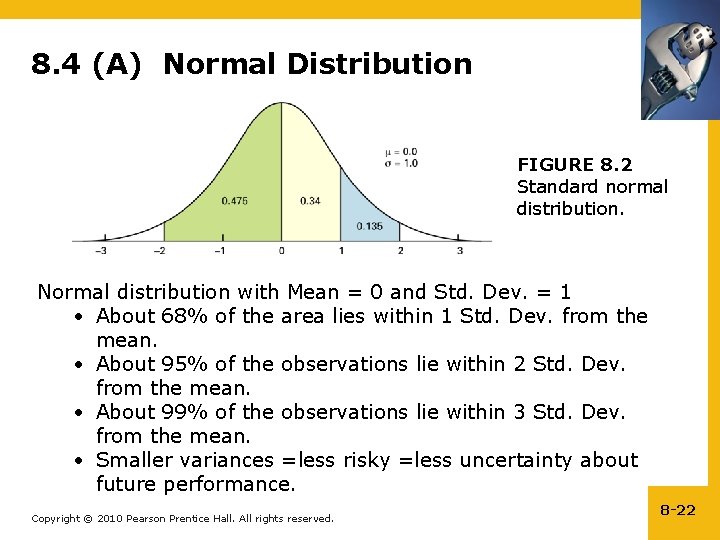
8. 4 (A) Normal Distribution FIGURE 8. 2 Standard normal distribution. Normal distribution with Mean = 0 and Std. Dev. = 1 • About 68% of the area lies within 1 Std. Dev. from the mean. • About 95% of the observations lie within 2 Std. Dev. from the mean. • About 99% of the observations lie within 3 Std. Dev. from the mean. • Smaller variances =less risky =less uncertainty about future performance. Copyright © 2010 Pearson Prentice Hall. All rights reserved. 8 -22

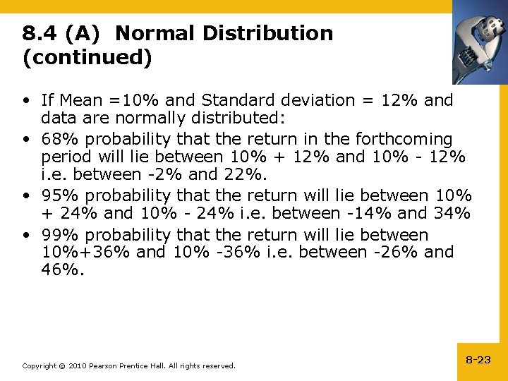
8. 4 (A) Normal Distribution (continued) • If Mean =10% and Standard deviation = 12% and data are normally distributed: • 68% probability that the return in the forthcoming period will lie between 10% + 12% and 10% - 12% i. e. between -2% and 22%. • 95% probability that the return will lie between 10% + 24% and 10% - 24% i. e. between -14% and 34% • 99% probability that the return will lie between 10%+36% and 10% -36% i. e. between -26% and 46%. Copyright © 2010 Pearson Prentice Hall. All rights reserved. 8 -23

Table 8. 2 Returns, Variances, and Standard Deviations of Investment Choices, 1950– 1999 Copyright © 2010 Pearson Prentice Hall. All rights reserved. 8 -24

8. 4 (A) Normal Distribution (continued) FIGURE 8. 3 Historical returns and standard deviations of bonds and stocks. T = Treasury bills, B = government bonds, L = large-company stocks, and S = small-company stocks. Over the past 5 decades (1950 -1999), riskier investment groups have earned higher returns and vice-versa. History shows that the higher the return one expects, the greater the risk (variability of return) that one would have to tolerate. Copyright © 2010 Pearson Prentice Hall. All rights reserved. 8 -25

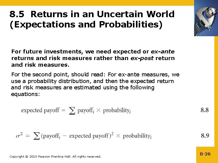
8. 5 Returns in an Uncertain World (Expectations and Probabilities) For future investments, we need expected or ex-ante returns and risk measures rather than ex-post return and risk measures. For the second point, should read: For ex-ante measures, we use a probability distribution, and then the expected return and risk measures are estimated using the following equations: Copyright © 2010 Pearson Prentice Hall. All rights reserved. 8 -26

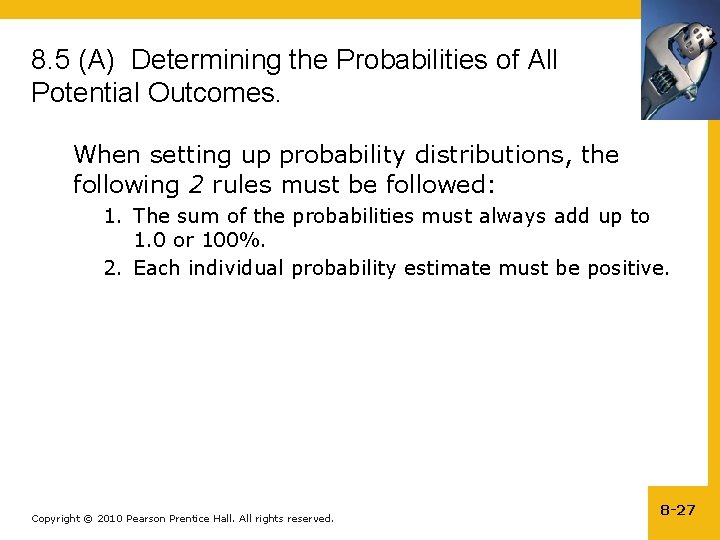
8. 5 (A) Determining the Probabilities of All Potential Outcomes. When setting up probability distributions, the following 2 rules must be followed: 1. The sum of the probabilities must always add up to 1. 0 or 100%. 2. Each individual probability estimate must be positive. Copyright © 2010 Pearson Prentice Hall. All rights reserved. 8 -27

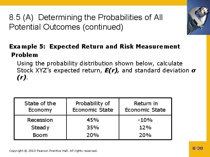
8. 5 (A) Determining the Probabilities of All Potential Outcomes (continued) Example 5: Expected Return and Risk Measurement Problem Using the probability distribution shown below, calculate Stock XYZ’s expected return, E(r), and standard deviation σ (r). State of the Economy Probability of Economic State Return in Economic State Recession Steady Boom 45% 35% 20% -10% 12% 20% Copyright © 2010 Pearson Prentice Hall. All rights reserved. 8 -28

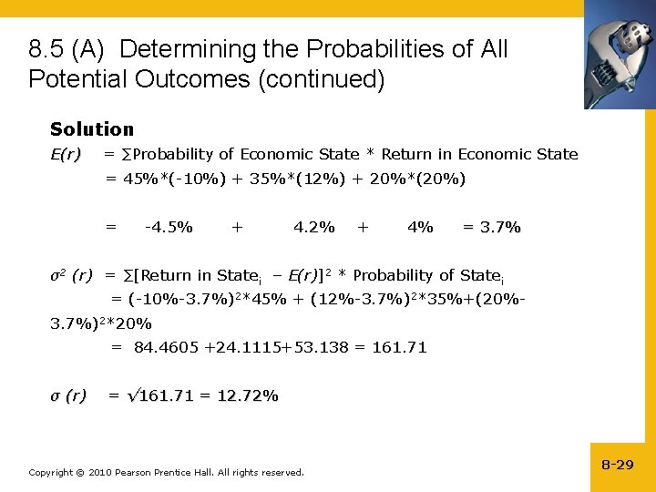
8. 5 (A) Determining the Probabilities of All Potential Outcomes (continued) Solution E(r) = ∑Probability of Economic State * Return in Economic State = 45%*(-10%) + 35%*(12%) + 20%*(20%) = -4. 5% + 4. 2% + 4% = 3. 7% σ2 (r) = ∑[Return in Statei – E(r)]2 * Probability of Statei = (-10%-3. 7%)2*45% + (12%-3. 7%)2*35%+(20%3. 7%)2*20% = 84. 4605 +24. 1115+53. 138 = 161. 71 σ (r) = √ 161. 71 = 12. 72% Copyright © 2010 Pearson Prentice Hall. All rights reserved. 8 -29

8. 6 The Risk-and-Return Trade-off • Investments must be analyzed in terms of both their return potential and in terms their risk or variability. • Historically, it has been proven that higher returns are accompanied by higher risks. Copyright © 2010 Pearson Prentice Hall. All rights reserved. 8 -30

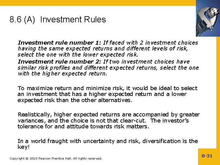
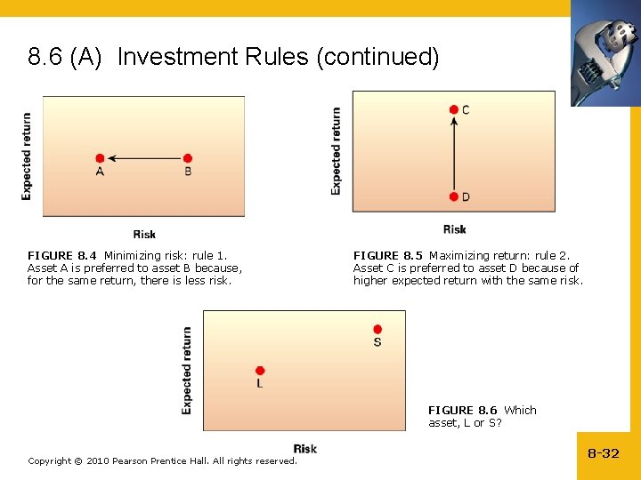
8. 6 (A) Investment Rules Investment rule number 1: If faced with 2 investment choices having the same expected returns and different levels of risk, select the one with the lower expected risk. Investment rule number 2: If two investment choices have similar risk profiles and different expected returns, select the one with the higher expected return. To maximize return and minimize risk, it would be ideal to select an investment that has a higher expected return and a lower expected risk than the other alternatives. Realistically, higher expected returns are accompanied by greater variances, and the choice is not that clear-cut. The investor’s tolerance for and attitude towards risk matters. In a world fraught with uncertainty and risk, diversification is the key! Copyright © 2010 Pearson Prentice Hall. All rights reserved. 8 -31

8. 6 (A) Investment Rules (continued) FIGURE 8. 4 Minimizing risk: rule 1. Asset A is preferred to asset B because, for the same return, there is less risk. FIGURE 8. 5 Maximizing return: rule 2. Asset C is preferred to asset D because of higher expected return with the same risk. FIGURE 8. 6 Which asset, L or S? Copyright © 2010 Pearson Prentice Hall. All rights reserved. 8 -32

8. 7 Diversification: Minimizing Risk or Uncertainty • Diversification is the spreading of wealth over a variety of investment opportunities so as to eliminate some risk. By dividing up one’s investments across many relatively low-correlated assets, companies, industries, and countries, it is possible to considerably reduce one’s exposure to risk. Copyright © 2010 Pearson Prentice Hall. All rights reserved. 8 -33

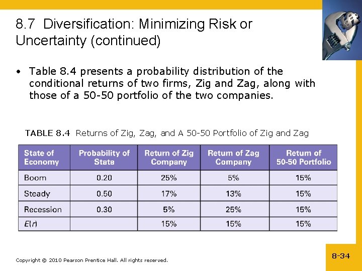
8. 7 Diversification: Minimizing Risk or Uncertainty (continued) • Table 8. 4 presents a probability distribution of the conditional returns of two firms, Zig and Zag, along with those of a 50 -50 portfolio of the two companies. TABLE 8. 4 Returns of Zig, Zag, and A 50 -50 Portfolio of Zig and Zag Copyright © 2010 Pearson Prentice Hall. All rights reserved. 8 -34

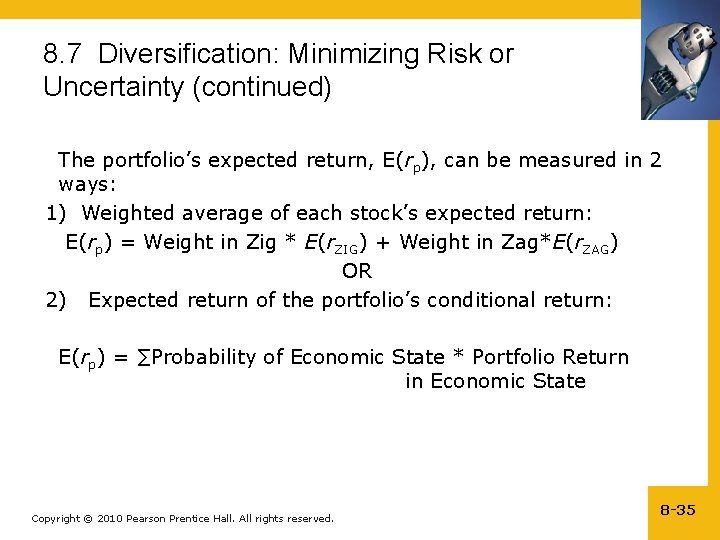
8. 7 Diversification: Minimizing Risk or Uncertainty (continued) The portfolio’s expected return, E(rp), can be measured in 2 ways: 1) Weighted average of each stock’s expected return: E(rp) = Weight in Zig * E(r. ZIG) + Weight in Zag*E(r. ZAG) OR 2) Expected return of the portfolio’s conditional return: E(rp) = ∑Probability of Economic State * Portfolio Return in Economic State Copyright © 2010 Pearson Prentice Hall. All rights reserved. 8 -35

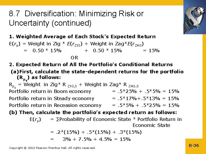
8. 7 Diversification: Minimizing Risk or Uncertainty (continued) 1. Weighted Average of Each Stock’s Expected Return E(rp) = Weight in Zig * E(r. ZIG) + Weight in Zag*E(r. ZAG) = 0. 50 * 15% + 0. 50 * 15% = 15% OR 2. Expected Return of All the Portfolio’s Conditional Returns (a)First, calculate the state-dependent returns for the portfolio (Rp ) as follows: s Rp = Weight in Zig* R ZIG, S + Weight in Zag* R ZAG, S s Portfolio return in Boom economy =. 5*25% +. 5*5% = 15% Portfolio return in Steady economy =. 5*17%+. 5*13% = 15% Portfolio return in Recession economy =. 5*5% +. 5*25% = 15% (b) Then, calculate the portfolio’s expected return as follows: E(rp) = ∑Probability of Economic State * Portfolio Return in Economic State =. 2*(15%) +. 5*(15%) +. 3*(15%) = 3% + 7. 5% + 4. 5% = 15% Copyright © 2010 Pearson Prentice Hall. All rights reserved. 8 -36

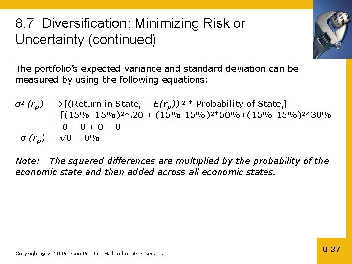
8. 7 Diversification: Minimizing Risk or Uncertainty (continued) The portfolio’s expected variance and standard deviation can be measured by using the following equations: σ2 (rp) = ∑[(Return in Statei – E(rp)) 2 * Probability of Statei] = [(15%– 15%)2*. 20 + (15%-15%)2*50%+(15%-15%)2*30% = 0 + 0 = 0 σ (rp) = √ 0 = 0% Note: The squared differences are multiplied by the probability of the economic state and then added across all economic states. Copyright © 2010 Pearson Prentice Hall. All rights reserved. 8 -37

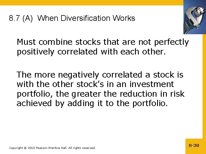
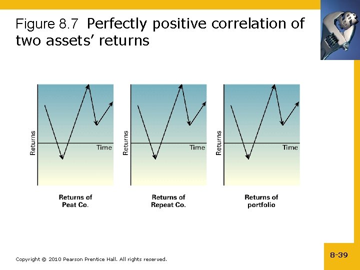
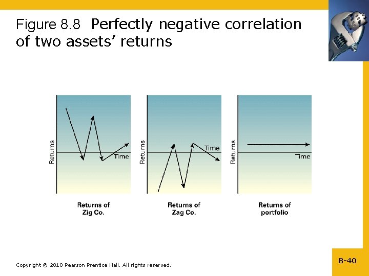
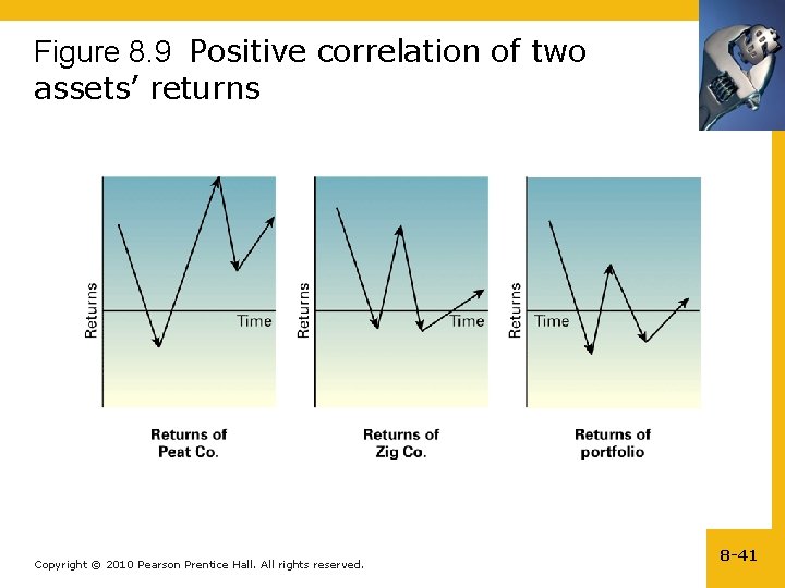
8. 7 (A) When Diversification Works Must combine stocks that are not perfectly positively correlated with each other. The more negatively correlated a stock is with the other stock’s in an investment portfolio, the greater the reduction in risk achieved by adding it to the portfolio. Copyright © 2010 Pearson Prentice Hall. All rights reserved. 8 -38

Figure 8. 7 Perfectly positive correlation of two assets’ returns Copyright © 2010 Pearson Prentice Hall. All rights reserved. 8 -39

Figure 8. 8 Perfectly negative correlation of two assets’ returns Copyright © 2010 Pearson Prentice Hall. All rights reserved. 8 -40

Figure 8. 9 Positive correlation of two assets’ returns Copyright © 2010 Pearson Prentice Hall. All rights reserved. 8 -41

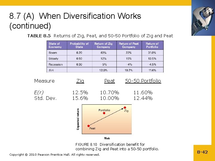
8. 7 (A) When Diversification Works (continued) TABLE 8. 5 Returns of Zig, Peat, and 50 -50 Portfolio of Zig and Peat Measure E(r) Std. Dev. Zig 12. 5% 15. 6% Peat 50 -50 Portfolio 10. 70% 10. 00% 11. 60% 12. 44% FIGURE 8. 10 Diversification benefit for combining Zig and Peat into a 50 -50 portfolio. Copyright © 2010 Pearson Prentice Hall. All rights reserved. 8 -42

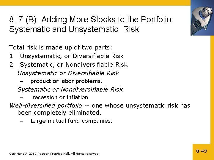
8. 7 (B) Adding More Stocks to the Portfolio: Systematic and Unsystematic Risk Total risk is made up of two parts: 1. Unsystematic, or Diversifiable Risk 2. Systematic, or Nondiversifiable Risk Unsystematic or Diversifiable Risk – product or labor problems. Systematic or Nondiversifiable Risk – recession or inflation Well-diversified portfolio -- one whose unsystematic risk has been completely eliminated. – Large mutual fund companies. Copyright © 2010 Pearson Prentice Hall. All rights reserved. 8 -43

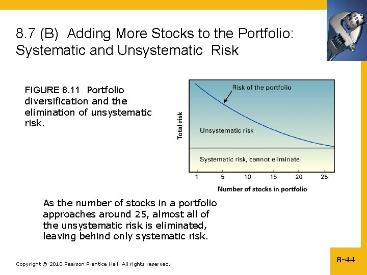
8. 7 (B) Adding More Stocks to the Portfolio: Systematic and Unsystematic Risk FIGURE 8. 11 Portfolio diversification and the elimination of unsystematic risk. As the number of stocks in a portfolio approaches around 25, almost all of the unsystematic risk is eliminated, leaving behind only systematic risk. Copyright © 2010 Pearson Prentice Hall. All rights reserved. 8 -44

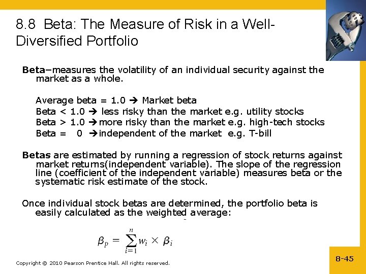
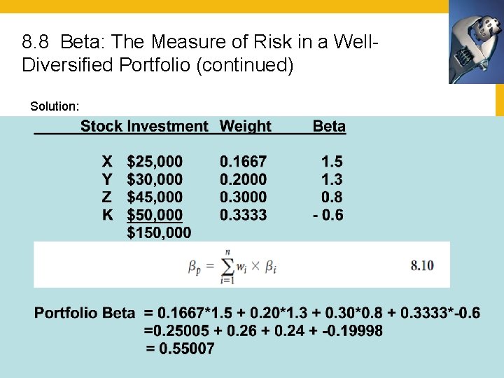
8. 8 Beta: The Measure of Risk in a Well. Diversified Portfolio Beta–measures the volatility of an individual security against the market as a whole. Average beta = 1. 0 Market beta Beta < 1. 0 less risky than the market e. g. utility stocks Beta > 1. 0 more risky than the market e. g. high-tech stocks Beta = 0 independent of the market e. g. T-bill Betas are estimated by running a regression of stock returns against market returns(independent variable). The slope of the regression line (coefficient of the independent variable) measures beta or the systematic risk estimate of the stock. Once individual stock betas are determined, the portfolio beta is easily calculated as the weighted average: Copyright © 2010 Pearson Prentice Hall. All rights reserved. 8 -45

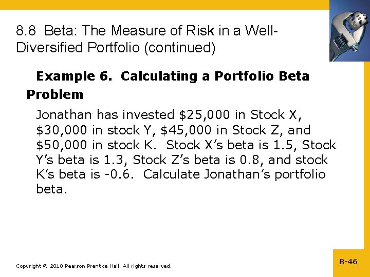
8. 8 Beta: The Measure of Risk in a Well. Diversified Portfolio (continued) Example 6. Calculating a Portfolio Beta Problem Jonathan has invested $25, 000 in Stock X, $30, 000 in stock Y, $45, 000 in Stock Z, and $50, 000 in stock K. Stock X’s beta is 1. 5, Stock Y’s beta is 1. 3, Stock Z’s beta is 0. 8, and stock K’s beta is -0. 6. Calculate Jonathan’s portfolio beta. Copyright © 2010 Pearson Prentice Hall. All rights reserved. 8 -46

8. 8 Beta: The Measure of Risk in a Well. Diversified Portfolio (continued) Solution: Copyright © 2010 Pearson Prentice Hall. All rights reserved. 8 -47

8. 8 Beta: The Measure of Risk in a Well. Diversified Portfolio (continued) 2 different measures of risk related to financial assets; standard deviation (or variance) and beta. Standard deviation--measure of the total risk of an asset, both its systematic and unsystematic risk. Beta--measure of an asset’s systematic risk. If an asset is part of a well-diversified portfolio, use beta as the measure of risk. If we do not have a well-diversified portfolio, it is more prudent to use standard deviation as the measure of risk for our asset. Copyright © 2010 Pearson Prentice Hall. All rights reserved. 8 -48

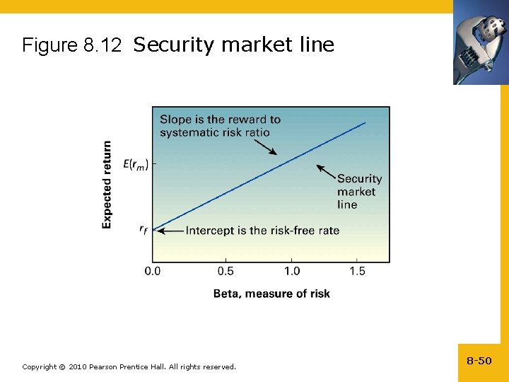
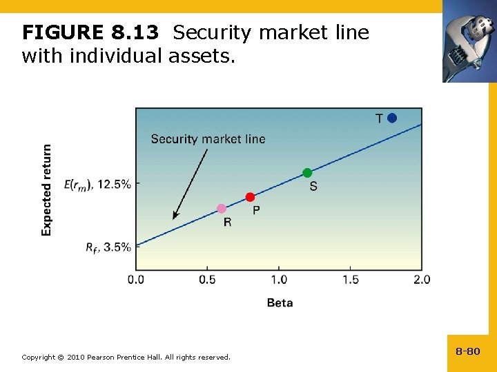
8. 9 The Capital Asset Pricing Model and the Security Market Line (SML) The SML shows the relationship between an asset’s required rate of return and its systematic risk measure, i. e. , beta. It is based on 3 assumptions: 1. There is a basic reward for waiting: the risk-free rate. consumption. 2. The greater the risk, the greater the expected reward. Investors expect to be proportionately compensated for bearing risk. 3. There is a consistent trade-off between risk and reward at all levels of risk. As risk doubles, so does the required rate of return, and vice-versa. These three assumptions imply that the SML is upward-sloping, has a constant slope (linear), and has the risk-free rate as its Yintercept. Copyright © 2010 Pearson Prentice Hall. All rights reserved. 8 -49

Figure 8. 12 Security market line Copyright © 2010 Pearson Prentice Hall. All rights reserved. 8 -50

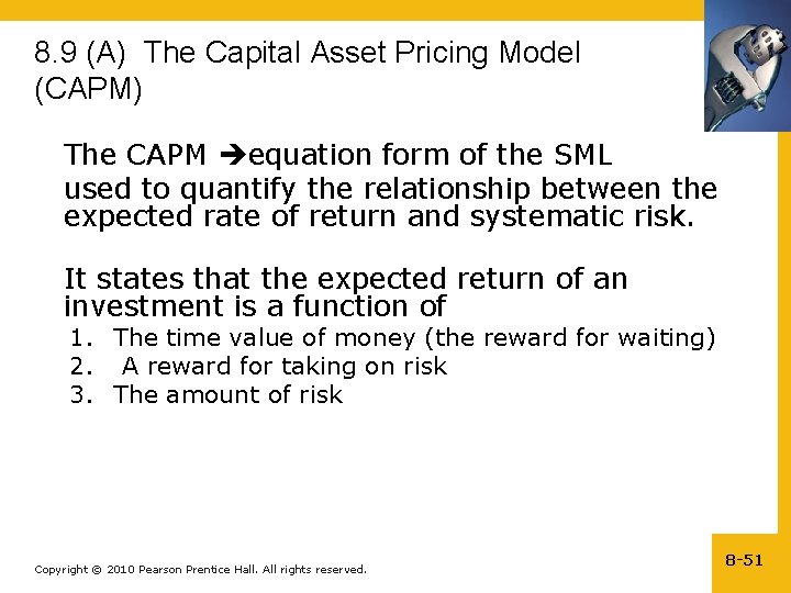
8. 9 (A) The Capital Asset Pricing Model (CAPM) The CAPM equation form of the SML used to quantify the relationship between the expected rate of return and systematic risk. It states that the expected return of an investment is a function of 1. The time value of money (the reward for waiting) 2. A reward for taking on risk 3. The amount of risk Copyright © 2010 Pearson Prentice Hall. All rights reserved. 8 -51

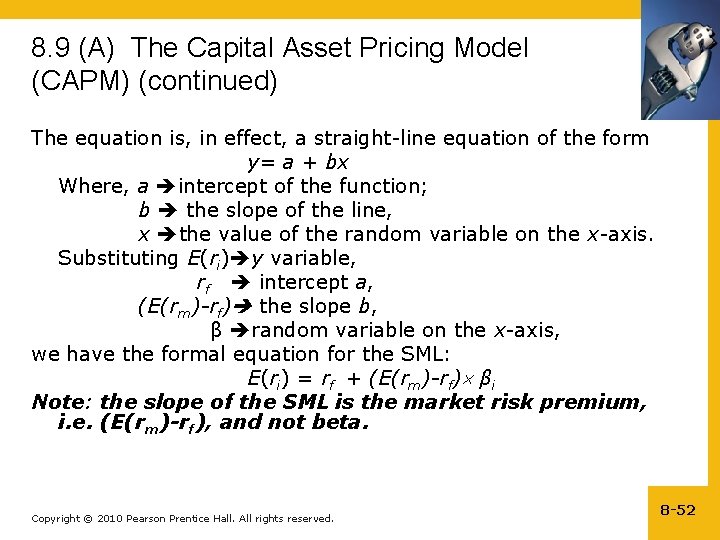
8. 9 (A) The Capital Asset Pricing Model (CAPM) (continued) The equation is, in effect, a straight-line equation of the form y= a + bx Where, a intercept of the function; b the slope of the line, x the value of the random variable on the x-axis. Substituting E(ri) y variable, rf intercept a, (E(rm)-rf) the slope b, β random variable on the x-axis, we have the formal equation for the SML: E(ri) = rf + (E(rm)-rf) βi Note: the slope of the SML is the market risk premium, i. e. (E(rm)-rf), and not beta. Copyright © 2010 Pearson Prentice Hall. All rights reserved. 8 -52

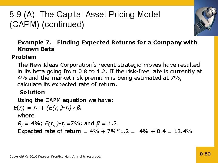
8. 9 (A) The Capital Asset Pricing Model (CAPM) (continued) Example 7. Finding Expected Returns for a Company with Known Beta Problem The New Ideas Corporation’s recent strategic moves have resulted in its beta going from 0. 8 to 1. 2. If the risk-free rate is currently at 4% and the market risk premium is being estimated at 7%, calculate its expected rate of return. Solution Using the CAPM equation we have: E(ri) = rf + (E(rm)-rf) βi where Rf = 4%; E(rm)-rf =7%; and β = 1. 2 Expected rate of return = 4% + 7%*1. 2 = 4% + 8. 4 = 12. 4% Copyright © 2010 Pearson Prentice Hall. All rights reserved. 8 -53

8. 9 (B) Application of the SML The SML has many practical applications such as…. 1. Determining the prevailing market or average risk premium 2. Determining the investment attractiveness of stocks. 3. Determining portfolio allocation weights and expected return. Copyright © 2010 Pearson Prentice Hall. All rights reserved. 8 -54

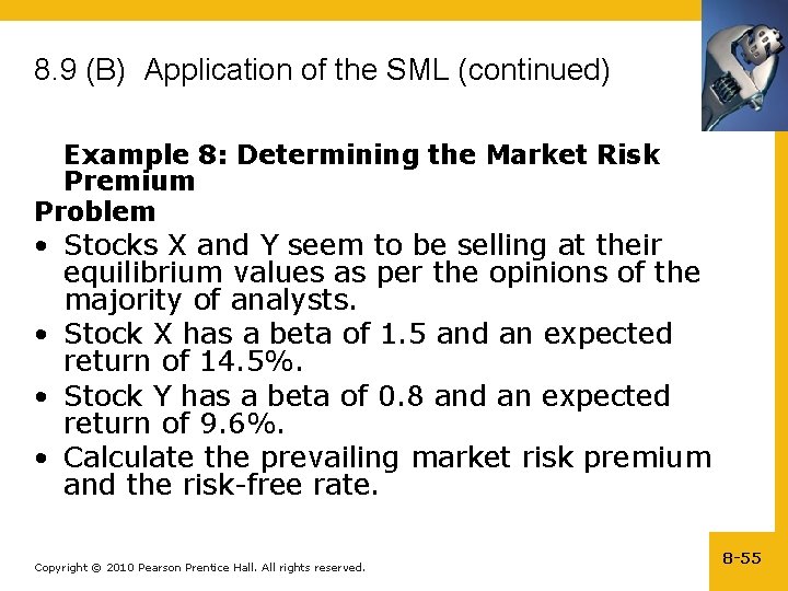
8. 9 (B) Application of the SML (continued) Example 8: Determining the Market Risk Premium Problem • Stocks X and Y seem to be selling at their equilibrium values as per the opinions of the majority of analysts. • Stock X has a beta of 1. 5 and an expected return of 14. 5%. • Stock Y has a beta of 0. 8 and an expected return of 9. 6%. • Calculate the prevailing market risk premium and the risk-free rate. Copyright © 2010 Pearson Prentice Hall. All rights reserved. 8 -55

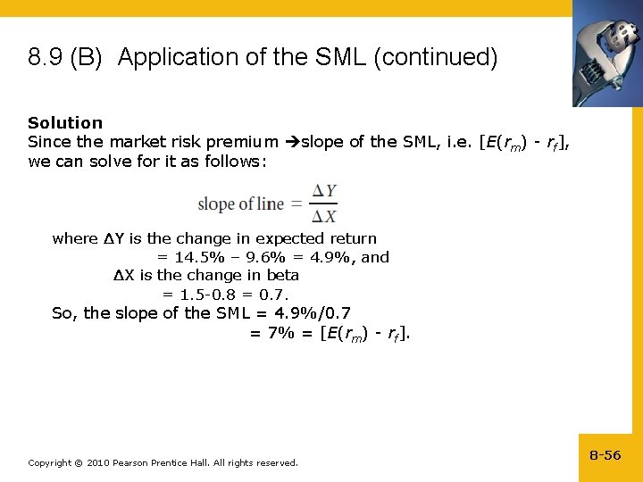
8. 9 (B) Application of the SML (continued) Solution Since the market risk premium slope of the SML, i. e. [E(rm) - rf], we can solve for it as follows: where ∆Y is the change in expected return = 14. 5% – 9. 6% = 4. 9%, and ∆X is the change in beta = 1. 5 -0. 8 = 0. 7. So, the slope of the SML = 4. 9%/0. 7 = 7% = [E(rm) - rf]. Copyright © 2010 Pearson Prentice Hall. All rights reserved. 8 -56

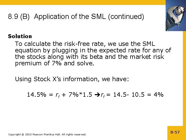
8. 9 (B) Application of the SML (continued) Solution To calculate the risk-free rate, we use the SML equation by plugging in the expected rate for any of the stocks along with its beta and the market risk premium of 7% and solve. Using Stock X’s information, we have: 14. 5% = rf + 7%*1. 5 rf = 14. 5 - 10. 5 = 4% Copyright © 2010 Pearson Prentice Hall. All rights reserved. 8 -57

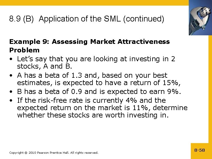
8. 9 (B) Application of the SML (continued) Example 9: Assessing Market Attractiveness Problem • Let’s say that you are looking at investing in 2 stocks, A and B. • A has a beta of 1. 3 and, based on your best estimates, is expected to have a return of 15%, • B has a beta of 0. 9 and is expected to earn 9%. • If the risk-free rate is currently 4% and the expected return on the market is 11%, determine whether these stocks are worth investing in. Copyright © 2010 Pearson Prentice Hall. All rights reserved. 8 -58

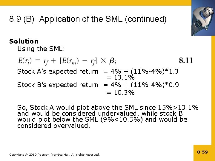
8. 9 (B) Application of the SML (continued) Solution Using the SML: Stock A’s expected return = 4% + (11%-4%)*1. 3 = 13. 1% Stock B’s expected return = 4% + (11%-4%)*0. 9 = 10. 3% So, Stock A would plot above the SML since 15%>13. 1% and would be considered undervalued, while stock B would plot below the SML (9%<10. 3%) and would be considered overvalued. Copyright © 2010 Pearson Prentice Hall. All rights reserved. 8 -59

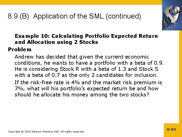
8. 9 (B) Application of the SML (continued) Example 10: Calculating Portfolio Expected Return and Allocation using 2 Stocks Problem Andrew has decided that given the current economic conditions, he wants to have a portfolio with a beta of 0. 9. He is considering Stock R with a beta of 1. 3 and Stock S with a beta of 0. 7 as the only 2 candidates for inclusion. If the risk-free rate is 4% and the market risk premium is 7%, what will his portfolio’s expected return be and how should he allocate his money among the two stocks? Copyright © 2010 Pearson Prentice Hall. All rights reserved. 8 -60

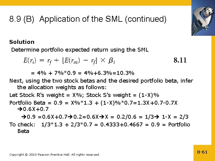
8. 9 (B) Application of the SML (continued) Solution Determine portfolio expected return using the SML = 4% + 7%*0. 9 = 4%+6. 3%=10. 3% Next, using the two stock betas and the desired portfolio beta, infer the allocation weights as follows: Let Stock R’s weight = X%; Stock S’s weight = (1 -X)% Portfolio Beta = 0. 9 = X%*1. 3 + (1 -X)%*0. 7=1. 3 X+0. 7 -0. 7 X 0. 6 X+0. 7 0. 9 =0. 6 X+0. 7 0. 2=0. 6 X X = 0. 2/0. 6 = 1/3 1 -X = 2/3 To check: 1/3*1. 3 + 2/3*0. 7 = 0. 4333+0. 4667 = 0. 9 = Portfolio Beta Copyright © 2010 Pearson Prentice Hall. All rights reserved. 8 -61

ADDITIONAL PROBLEMS WITH ANSWERS Problem 1 Comparing HPRs, APRs and EARs: Two years ago, Jim bought 100 shares of IBM stock at $50 per share, and just sold them for $65 per share after receiving dividends worth $3 per share over the two year holding period. Mary, bought 5 ounces of gold at $800 per ounce, three months ago , and just sold it for $1000 per ounce. Calculate each investor’s HPR, APR, and EAR and comment on your findings. Copyright © 2010 Pearson Prentice Hall. All rights reserved. 8 -62

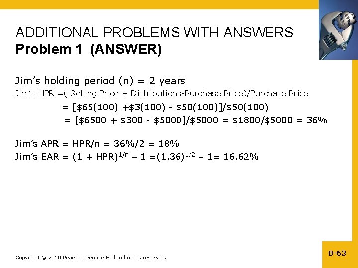
ADDITIONAL PROBLEMS WITH ANSWERS Problem 1 (ANSWER) Jim’s holding period (n) = 2 years Jim’s HPR =( Selling Price + Distributions-Purchase Price)/Purchase Price = [$65(100) +$3(100) - $50(100)]/$50(100) = [$6500 + $300 - $5000]/$5000 = $1800/$5000 = 36% Jim’s APR = HPR/n = 36%/2 = 18% Jim’s EAR = (1 + HPR)1/n – 1 =(1. 36)1/2 – 1= 16. 62% Copyright © 2010 Pearson Prentice Hall. All rights reserved. 8 -63

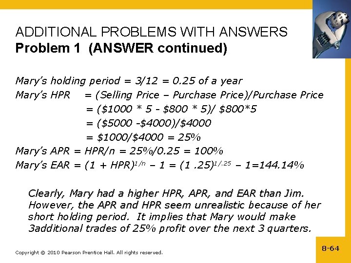
ADDITIONAL PROBLEMS WITH ANSWERS Problem 1 (ANSWER continued) Mary’s holding period = 3/12 = 0. 25 of a year Mary’s HPR = (Selling Price – Purchase Price)/Purchase Price = ($1000 * 5 - $800 * 5)/ $800*5 = ($5000 -$4000)/$4000 = $1000/$4000 = 25% Mary’s APR = HPR/n = 25%/0. 25 = 100% Mary’s EAR = (1 + HPR)1/n – 1 = (1. 25)1/. 25 – 1=144. 14% Clearly, Mary had a higher HPR, APR, and EAR than Jim. However, the APR and HPR seem unrealistic because of her the APR and HPR seem unrealistic short holding period. It implies that Mary would make 3 additional trades of 25% profit over the next 3 quarters. Copyright © 2010 Pearson Prentice Hall. All rights reserved. 8 -64

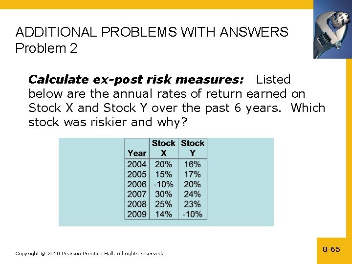
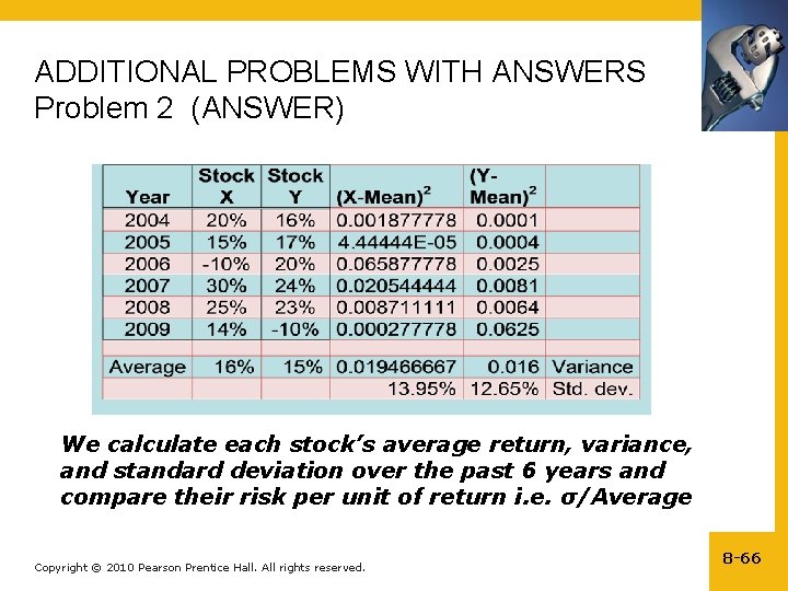
ADDITIONAL PROBLEMS WITH ANSWERS Problem 2 Calculate ex-post risk measures: Listed below are the annual rates of return earned on Stock X and Stock Y over the past 6 years. Which stock was riskier and why? Copyright © 2010 Pearson Prentice Hall. All rights reserved. 8 -65

ADDITIONAL PROBLEMS WITH ANSWERS Problem 2 (ANSWER) We calculate each stock’s average return, variance, and standard deviation over the past 6 years and compare their risk per unit of return i. e. σ/Average Copyright © 2010 Pearson Prentice Hall. All rights reserved. 8 -66

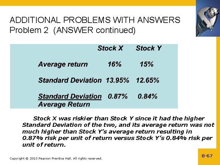
ADDITIONAL PROBLEMS WITH ANSWERS Problem 2 (ANSWER continued) Stock X was riskier than Stock Y since it had the higher Standard Deviation of the two, and its average return was not much higher than Stock Y’s average return resulting in 0. 87% risk per unit of return versus Stock Y’s 0. 84% risk per unit of return. Copyright © 2010 Pearson Prentice Hall. All rights reserved. 8 -67

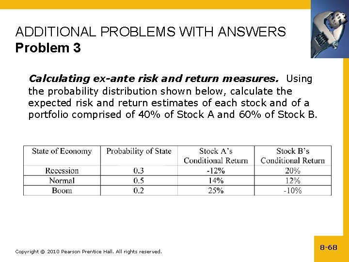
ADDITIONAL PROBLEMS WITH ANSWERS Problem 3 Calculating ex-ante risk and return measures. Using the probability distribution shown below, calculate the expected risk and return estimates of each stock and of a portfolio comprised of 40% of Stock A and 60% of Stock B. Copyright © 2010 Pearson Prentice Hall. All rights reserved. 8 -68

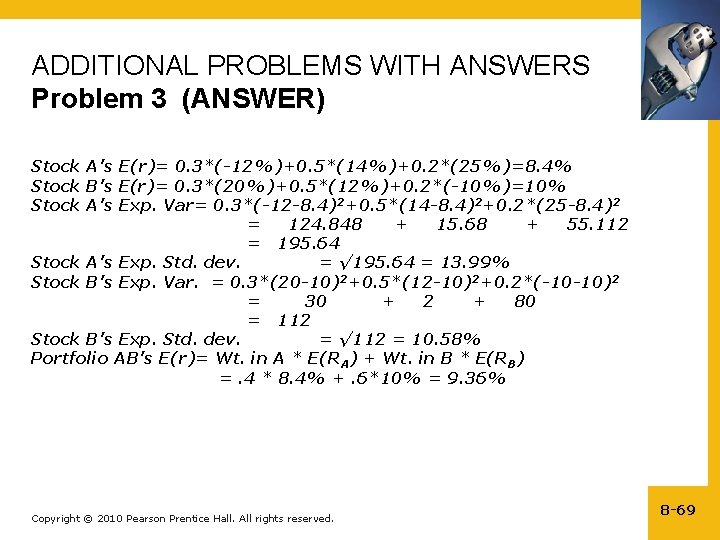
ADDITIONAL PROBLEMS WITH ANSWERS Problem 3 (ANSWER) Stock A’s E(r)= 0. 3*(-12%)+0. 5*(14%)+0. 2*(25%)=8. 4% Stock B’s E(r)= 0. 3*(20%)+0. 5*(12%)+0. 2*(-10%)=10% Stock A’s Exp. Var= 0. 3*(-12 -8. 4)2+0. 5*(14 -8. 4)2+0. 2*(25 -8. 4)2 = 124. 848 + 15. 68 + 55. 112 = 195. 64 Stock A’s Exp. Std. dev. = √ 195. 64 = 13. 99% Stock B’s Exp. Var. = 0. 3*(20 -10)2+0. 5*(12 -10)2+0. 2*(-10 -10)2 = 30 + 2 + 80 = 112 Stock B’s Exp. Std. dev. = √ 112 = 10. 58% Portfolio AB’s E(r)= Wt. in A * E(RA) + Wt. in B * E(RB) =. 4 * 8. 4% +. 6*10% = 9. 36% Copyright © 2010 Pearson Prentice Hall. All rights reserved. 8 -69

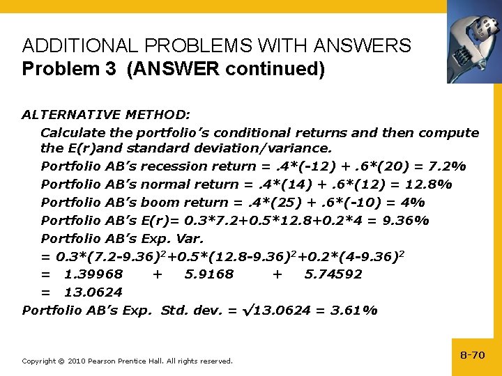
ADDITIONAL PROBLEMS WITH ANSWERS Problem 3 (ANSWER continued) ALTERNATIVE METHOD: Calculate the portfolio’s conditional returns and then compute the E(r)and standard deviation/variance. Portfolio AB’s recession return =. 4*(-12) +. 6*(20) = 7. 2% Portfolio AB’s normal return =. 4*(14) +. 6*(12) = 12. 8% Portfolio AB’s boom return =. 4*(25) +. 6*(-10) = 4% Portfolio AB’s E(r)= 0. 3*7. 2+0. 5*12. 8+0. 2*4 = 9. 36% Portfolio AB’s Exp. Var. = 0. 3*(7. 2 -9. 36)2+0. 5*(12. 8 -9. 36)2+0. 2*(4 -9. 36)2 = 1. 39968 + 5. 9168 + 5. 74592 = 13. 0624 Portfolio AB’s Exp. Std. dev. = √ 13. 0624 = 3. 61% Copyright © 2010 Pearson Prentice Hall. All rights reserved. 8 -70

ADDITIONAL PROBLEMS WITH ANSWERS Problem 4 Calculate a portfolio’s expected rate of return using the CAPM Annie is curious to know what her portfolio’s CAPMbased expected rate of return should be. After doing some research, she figures out the market values and betas of each of her 5 stocks (shown below) and is told by her consultant that the risk-free rate is 3% and the market risk premium is 8%. Help Annie calculate her portfolio’s expected rate of return. Copyright © 2010 Pearson Prentice Hall. All rights reserved. 8 -71

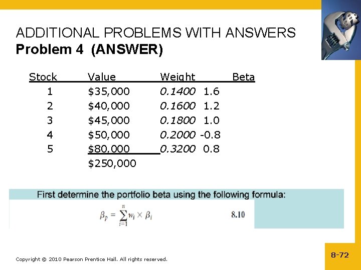
ADDITIONAL PROBLEMS WITH ANSWERS Problem 4 (ANSWER) Stock 1 2 3 4 5 Value $35, 000 $40, 000 $45, 000 $50, 000 $80, 000 $250, 000 Weight 0. 1400 1. 6 0. 1600 1. 2 0. 1800 1. 0 0. 2000 -0. 8 0. 3200 0. 8 Beta Copyright © 2010 Pearson Prentice Hall. All rights reserved. 8 -72

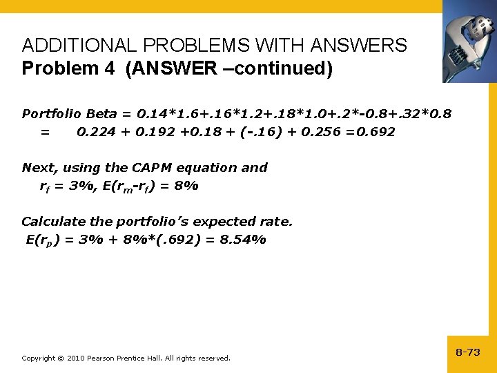
ADDITIONAL PROBLEMS WITH ANSWERS Problem 4 (ANSWER –continued) Portfolio Beta = 0. 14*1. 6+. 16*1. 2+. 18*1. 0+. 2*-0. 8+. 32*0. 8 = 0. 224 + 0. 192 +0. 18 + (-. 16) + 0. 256 =0. 692 Next, using the CAPM equation and rf = 3%, E(rm-rf) = 8% Calculate the portfolio’s expected rate. E(rp) = 3% + 8%*(. 692) = 8. 54% Copyright © 2010 Pearson Prentice Hall. All rights reserved. 8 -73

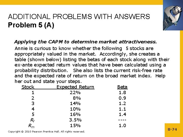
ADDITIONAL PROBLEMS WITH ANSWERS Problem 5 (A) Applying the CAPM to determine market attractiveness. Annie is curious to know whether the following 5 stocks are appropriately valued in the market. Accordingly, she creates a table (shown below) listing the betas of each stock along with their ex-ante expected return values that have been calculated using a probability distribution. She also lists the current risk-free rate and the expected rate of return on the broad market index. Help her out and state your steps. Stock Expected Return Beta 1 22% 1. 8 2 8% 0. 9 3 14% 1. 2 4 10% 1. 1 5 16% 1. 4 Rf 3. 5% --- Rm 15% 1. 0 Copyright © 2010 Pearson Prentice Hall. All rights reserved. 8 -74

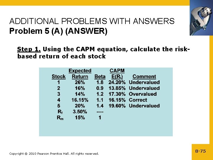
ADDITIONAL PROBLEMS WITH ANSWERS Problem 5 (A) (ANSWER) Step 1. Using the CAPM equation, calculate the riskbased return of each stock Copyright © 2010 Pearson Prentice Hall. All rights reserved. 8 -75

ADDITIONAL PROBLEMS WITH ANSWERS Problem 5 (B) If Annie wants to form a 2 -stock portfolio of the most undervalued stocks with a beta of 1. 3, by how much will she have to weight each of the stocks? Copyright © 2010 Pearson Prentice Hall. All rights reserved. 8 -76

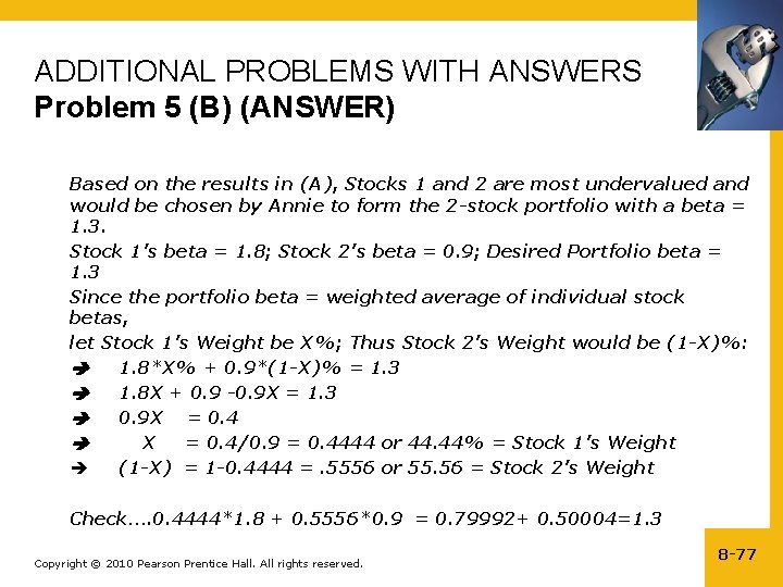
ADDITIONAL PROBLEMS WITH ANSWERS Problem 5 (B) (ANSWER) Based on the results in (A), Stocks 1 and 2 are most undervalued and would be chosen by Annie to form the 2 -stock portfolio with a beta = 1. 3. Stock 1’s beta = 1. 8; Stock 2’s beta = 0. 9; Desired Portfolio beta = 1. 3 Since the portfolio beta = weighted average of individual stock betas, let Stock 1’s Weight be X%; Thus Stock 2’s Weight would be (1 -X)%: 1. 8*X% + 0. 9*(1 -X)% = 1. 3 1. 8 X + 0. 9 -0. 9 X = 1. 3 0. 9 X = 0. 4 X = 0. 4/0. 9 = 0. 4444 or 44. 44% = Stock 1’s Weight (1 -X) = 1 -0. 4444 =. 5556 or 55. 56 = Stock 2’s Weight Check…. 0. 4444*1. 8 + 0. 5556*0. 9 = 0. 79992+ 0. 50004=1. 3 Copyright © 2010 Pearson Prentice Hall. All rights reserved. 8 -77

TABLE 8. 1 Year-by-Year Returns and Decade Averages, 1950– 1999 Copyright © 2010 Pearson Prentice Hall. All rights reserved. 8 -78

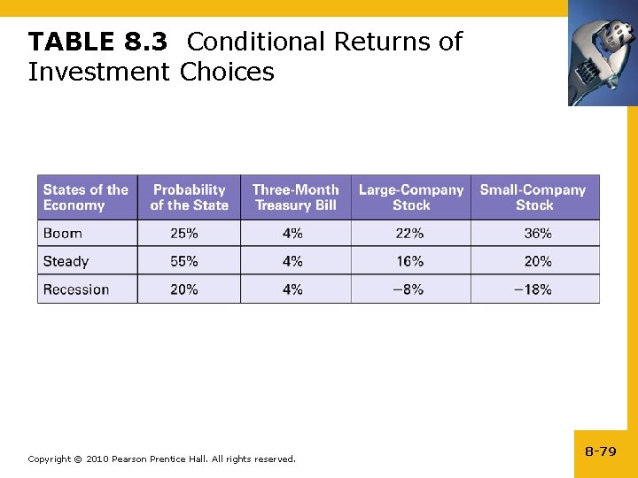
TABLE 8. 3 Conditional Returns of Investment Choices Copyright © 2010 Pearson Prentice Hall. All rights reserved. 8 -79

FIGURE 8. 13 Security market line with individual assets. Copyright © 2010 Pearson Prentice Hall. All rights reserved. 8 -80