Chapter 20 Model Predictive Control Model Predictive Control

Chapter 20 Model Predictive Control • Model Predictive Control (MPC) – regulatory controls that use an explicit dynamic model of the response of process variables to changes in manipulated variables to calculate control “moves”. • Control moves are intended to force the process variables to follow a pre-specified trajectory from the current operating point to the target. • Base control action on current measurements and future predictions. 1

Chapter 20 DMC – dynamic matrix control became MPC – model predictive control • Optimal controller is based on minimizing error from set point • Basic version uses linear model, but there are many possible models • Corrections for unmeasured disturbances, model errors are included • Single step and multi-step versions • Treats multivariable control, feedforward control 2

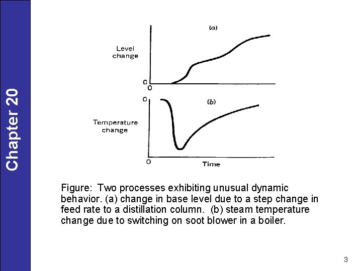
Chapter 20 Figure: Two processes exhibiting unusual dynamic behavior. (a) change in base level due to a step change in feed rate to a distillation column. (b) steam temperature change due to switching on soot blower in a boiler. 3

Chapter 20 When Should Predictive Control be Used? 1. Processes are difficult to control with standard PID algorithm – long time constants, substantial time delays, inverse response, etc. 2. There is substantial dynamic interaction among controls, i. e. , more than one manipulated variable has a significant effect on an important process variable. 3. Constraints (limits) on process variables and manipulated variables are important for normal control. 4

Chapter 20 Overall Objectives of Model Predictive Control 1. Prevent violations of input and output constraints. 2. Drive some output variables to their optimal set points, while maintaining other outputs within specified ranges. 3. Prevent excessive movement of the input variables. 4. If a sensor or actuator is not available, control as much of the process as possible. 5

Model Predictive Control: Basic Concepts 1. Future values of output variables are predicted using a dynamic model of the process and current measurements. Chapter 20 • 2. 3. The control calculations are based on both future predictions and current measurements. The manipulated variables, u(k), at the k-th sampling instant are calculated so that they minimize an objective function, J. • • 4. 5. Unlike time delay compensation methods, the predictions are made for more than one time delay ahead. Example: Minimize the sum of the squares of the deviations between predicted future outputs and specific reference trajectory. The reference trajectory is based on set points calculated using RTO. Inequality & equality constraints, and measured disturbances are included in the control calculations. The calculated manipulated variables are implemented as set point for lower level control loops. (cf. cascade control). 6

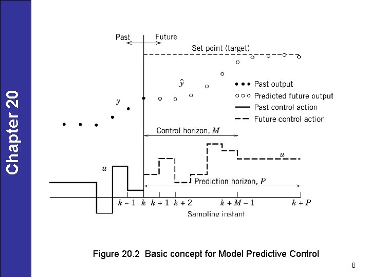
Model Predictive Control: Calculations Chapter 20 1. At the k-th sampling instant, the values of the manipulated variables, u, at the next M sampling instants, {u(k), u(k+1), …, u(k+M -1)} are calculated. • This set of M “control moves” is calculated so as to minimize the predicted deviations from the reference trajectory over the next P sampling instants while satisfying the constraints. • Typically, an LP or QP problem is solved at each sampling instant. • Terminology: M = control horizon, P = prediction horizon 2. Then the first “control move”, u(k), is implemented. 3. At the next sampling instant, k+1, the M-step control policy is re -calculated for the next M sampling instants, k+1 to k+M, and implement the first control move, u(k+1). 4. Then Steps 1 and 2 are repeated for subsequent sampling instants. Note: This approach is an example of a receding horizon approach. 7

Chapter 20 Figure 20. 2 Basic concept for Model Predictive Control 8

Chapter 20 When Should Predictive Control be Used? 1. Processes are difficult to control with standard PID algorithm (e. g. , large time constants, substantial time delays, inverse response, etc. 2. There is significant process interactions between u and y. • i. e. , more than one manipulated variable has a significant effect on an important process variable. 3. Constraints (limits) on process variables and manipulated variables are important for normal control. Terminology: • y ↔ CV, u ↔ MV, d ↔ DV 9

Model Predictive Control Originated in 1980 s Chapter 20 • Techniques developed by industry: 1. Dynamic Matrix Control (DMC) • Shell Development Co. : Cutler and Ramaker (1980), • Cutler later formed DMC, Inc. • DMC acquired by Aspentech in 1997. 2. Model Algorithmic Control (MAC) • ADERSA/GERBIOS, Richalet et al. (1978) in France. • Over 5000 applications of MPC since 1980 Reference: Qin and Badgwell, 1998 and 2003). 10

Dynamic Models for Model Predictive Control Chapter 20 • Could be either: 1. Physical or empirical (but usually empirical) 2. Linear or nonlinear (but usually linear) • Typical linear models used in MPC: 1. Step response models 2. Transfer function models 3. State-space models • Note: Can convert one type of linear model (above) to the other types. 11

General Characteristics Chapter 20 • Targets (set points) selected by real-time optimization software based on current operating and economic conditions • Minimize square of deviations between predicted future outputs and specific reference trajectory to new targets • Discrete step response model • Framework handles multiple input, multiple output (MIMO) control problems. 12

Chapter 20 • Can include equality and inequality constraints on controlled and manipulated variables • Solves a quadratic programming problem at each sampling instant • Disturbance is estimated by comparing the actual controlled variable with the model prediction • Usually implements the first move out of M calculated moves 13

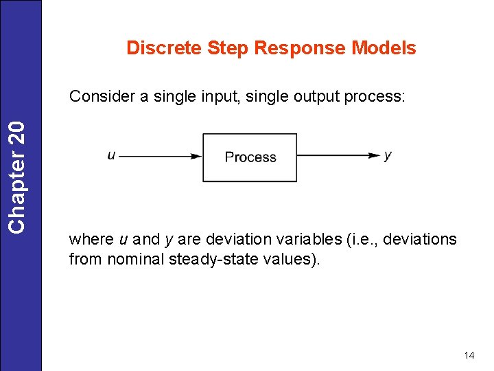
Discrete Step Response Models Chapter 20 Consider a single input, single output process: where u and y are deviation variables (i. e. , deviations from nominal steady-state values). 14

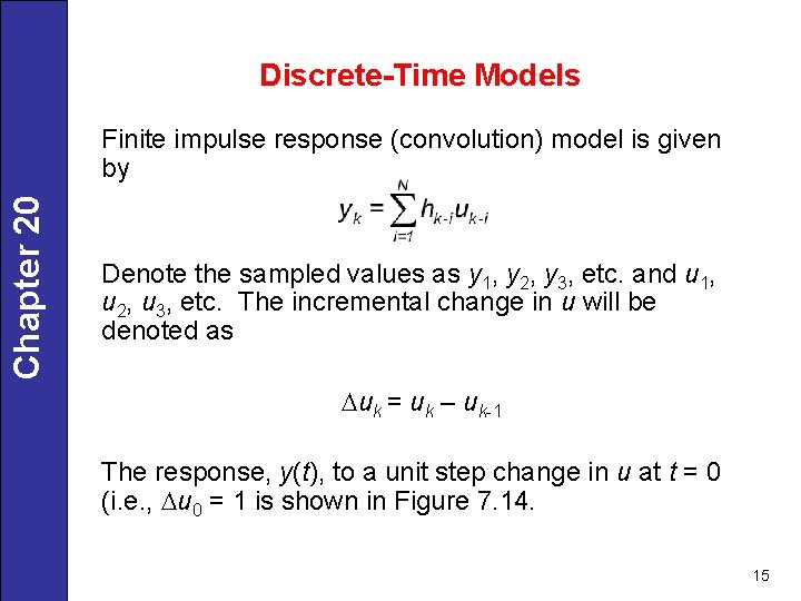
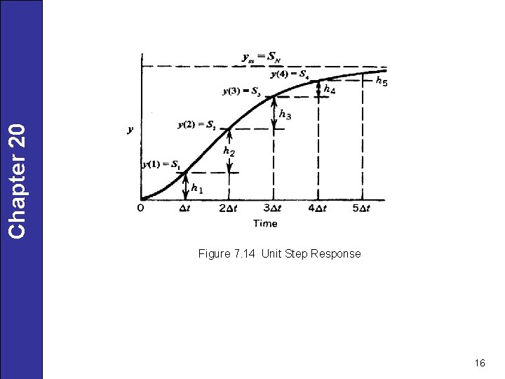
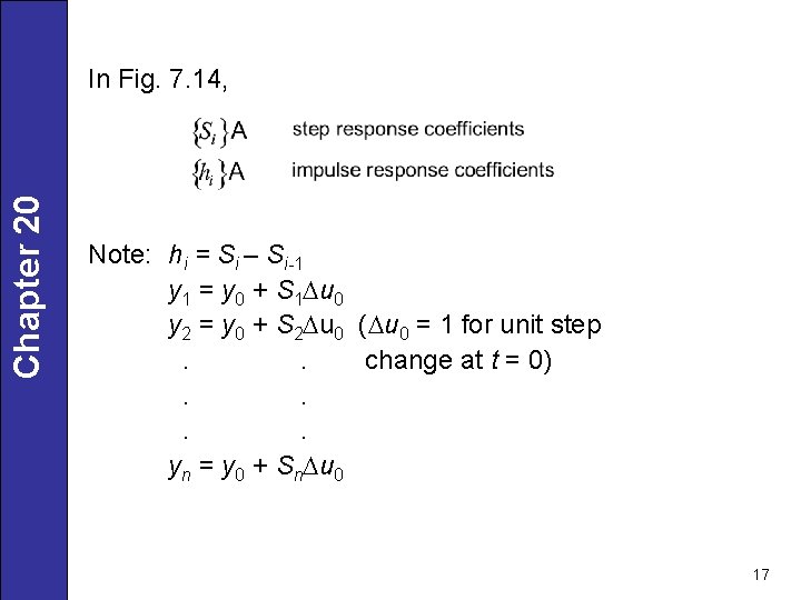
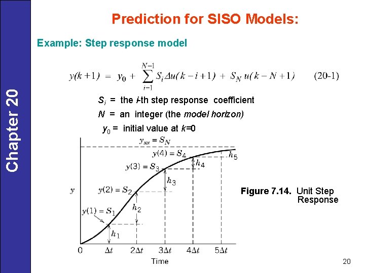
Discrete-Time Models Chapter 20 Finite impulse response (convolution) model is given by Denote the sampled values as y 1, y 2, y 3, etc. and u 1, u 2, u 3, etc. The incremental change in u will be denoted as Duk = uk – uk-1 The response, y(t), to a unit step change in u at t = 0 (i. e. , Du 0 = 1 is shown in Figure 7. 14. 15

Chapter 20 Figure 7. 14 Unit Step Response 16

Chapter 20 In Fig. 7. 14, Note: hi = Si – Si-1 y 1 = y 0 + S 1 Du 0 y 2 = y 0 + S 2 Du 0 (Du 0 = 1 for unit step. . change at t = 0). . yn = y 0 + Sn. Du 0 17

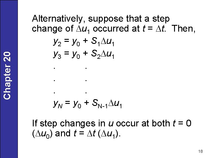
Chapter 20 Alternatively, suppose that a step change of Du 1 occurred at t = Dt. Then, y 2 = y 0 + S 1 Du 1 y 3 = y 0 + S 2 Du 1. . . y. N = y 0 + SN-1 Du 1 If step changes in u occur at both t = 0 (Du 0) and t = Dt (Du 1). 18

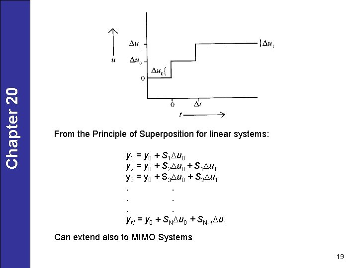
Chapter 20 From the Principle of Superposition for linear systems: y 1 = y 0 + S 1 Du 0 y 2 = y 0 + S 2 Du 0 + S 1 Du 1 y 3 = y 0 + S 3 Du 0 + S 2 Du 1. . . y. N = y 0 + SNDu 0 + SN-1 Du 1 Can extend also to MIMO Systems 19

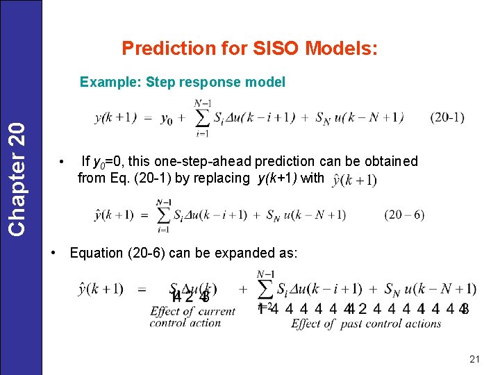
Prediction for SISO Models: Chapter 20 Example: Step response model Si = the i-th step response coefficient N = an integer (the model horizon) y 0 = initial value at k=0 Figure 7. 14. Unit Step Response 20

Prediction for SISO Models: Chapter 20 Example: Step response model • If y 0=0, this one-step-ahead prediction can be obtained from Eq. (20 -1) by replacing y(k+1) with • Equation (20 -6) can be expanded as: 21

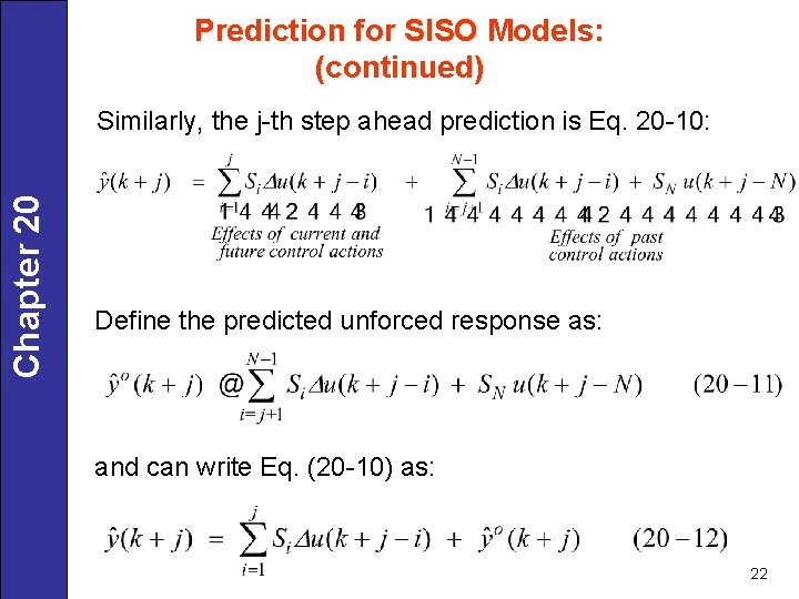
Prediction for SISO Models: (continued) Chapter 20 Similarly, the j-th step ahead prediction is Eq. 20 -10: Define the predicted unforced response as: and can write Eq. (20 -10) as: 22

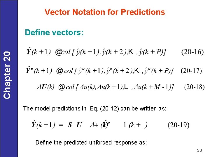
Vector Notation for Predictions Chapter 20 Define vectors: The model predictions in Eq. (20 -12) can be written as: Define the predicted unforced response as: 23

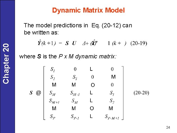
Dynamic Matrix Model Chapter 20 The model predictions in Eq. (20 -12) can be written as: where S is the P x M dynamic matrix: 24

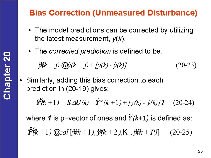
Bias Correction (Unmeasured Disturbance) Chapter 20 • The model predictions can be corrected by utilizing the latest measurement, y(k). • The corrected prediction is defined to be: • Similarly, adding this bias correction to each prediction in (20 -19) gives: 25

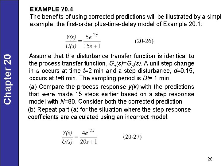
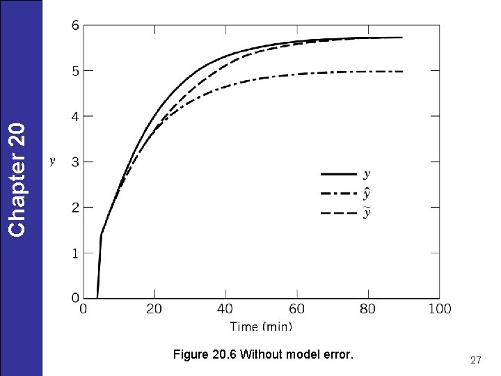
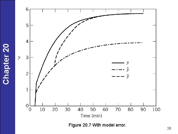
Chapter 20 EXAMPLE 20. 4 The benefits of using corrected predictions will be illustrated by a simpl example, the first-order plus-time-delay model of Example 20. 1: Assume that the disturbance transfer function is identical to the process transfer function, Gd(s)=Gp(s). A unit step change in u occurs at time t=2 min and a step disturbance, d=0. 15, occurs at t=8 min. The sampling period is Dt= 1 min. (a) Compare the process response y(k) with the predictions that were made 15 steps earlier based on a step response model with N=80. Consider both the corrected prediction (b) Repeat part (a) for the situation where the step response coefficients are calculated using an incorrect model: 26

Chapter 20 Figure 20. 6 Without model error. 27

Chapter 20 Figure 20. 7 With model error. 28

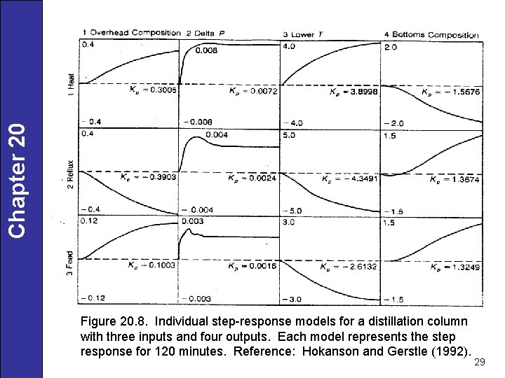
Chapter 20 Figure 20. 8. Individual step-response models for a distillation column with three inputs and four outputs. Each model represents the step response for 120 minutes. Reference: Hokanson and Gerstle (1992). 29

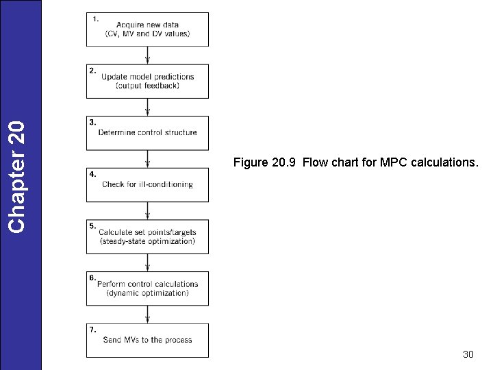
Chapter 20 Figure 20. 9 Flow chart for MPC calculations. 30

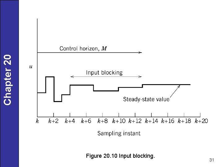
Chapter 20 Figure 20. 10 Input blocking. 31

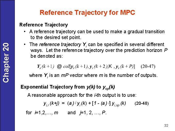
Chapter 20 Reference Trajectory for MPC Reference Trajectory • A reference trajectory can be used to make a gradual transition to the desired set point. • The reference trajectory Yr can be specified in several different ways. Let the reference trajectory over the prediction horizon P be denoted as: where Yr is an m. P vector where m is the number of outputs. Exponential Trajectory from y(k) to ysp(k) A reasonable approach for the i-th output is to use: yi, r (k+j) = (ai) j yi (k) + [1 - (ai) j] yi, sp (k) for i=1, 2, …, m (20 -48) and j=1, 2, …, P. 32

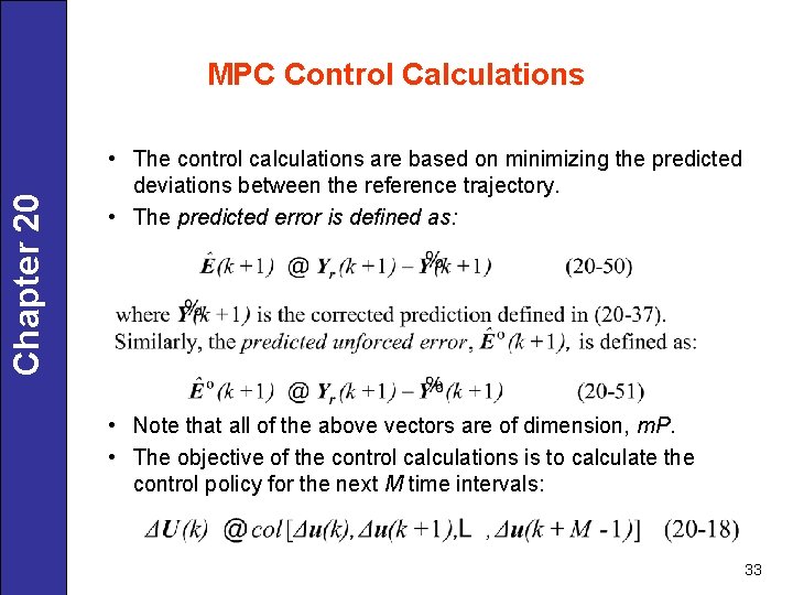
Chapter 20 MPC Control Calculations • The control calculations are based on minimizing the predicted deviations between the reference trajectory. • The predicted error is defined as: • Note that all of the above vectors are of dimension, m. P. • The objective of the control calculations is to calculate the control policy for the next M time intervals: 33

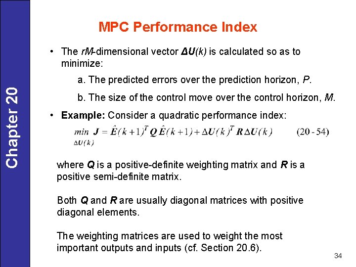
MPC Performance Index • The r. M-dimensional vector ΔU(k) is calculated so as to minimize: Chapter 20 a. The predicted errors over the prediction horizon, P. b. The size of the control move over the control horizon, M. • Example: Consider a quadratic performance index: where Q is a positive-definite weighting matrix and R is a positive semi-definite matrix. Both Q and R are usually diagonal matrices with positive diagonal elements. The weighting matrices are used to weight the most important outputs and inputs (cf. Section 20. 6). 34

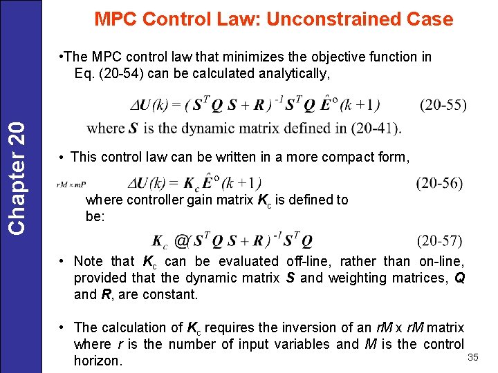
MPC Control Law: Unconstrained Case Chapter 20 • The MPC control law that minimizes the objective function in Eq. (20 -54) can be calculated analytically, • This control law can be written in a more compact form, where controller gain matrix Kc is defined to be: • Note that Kc can be evaluated off-line, rather than on-line, provided that the dynamic matrix S and weighting matrices, Q and R, are constant. • The calculation of Kc requires the inversion of an r. M x r. M matrix where r is the number of input variables and M is the control 35 horizon.

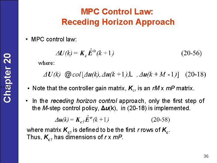
MPC Control Law: Receding Horizon Approach Chapter 20 • MPC control law: . where: • Note that the controller gain matrix, Kc, is an r. M x m. P matrix. • In the receding horizon control approach, only the first step of the M-step control policy, Δu(k), in (20 -18) is implemented. where matrix Kc 1 is defined to be the first r rows of Kc. Thus, Kc 1 has dimensions of r x m. P. 36

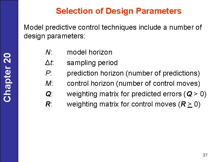
Selection of Design Parameters Chapter 20 Model predictive control techniques include a number of design parameters: N: Δt: P: M: Q: R: model horizon sampling period prediction horizon (number of predictions) control horizon (number of control moves) weighting matrix for predicted errors (Q > 0) weighting matrix for control moves (R > 0) 37

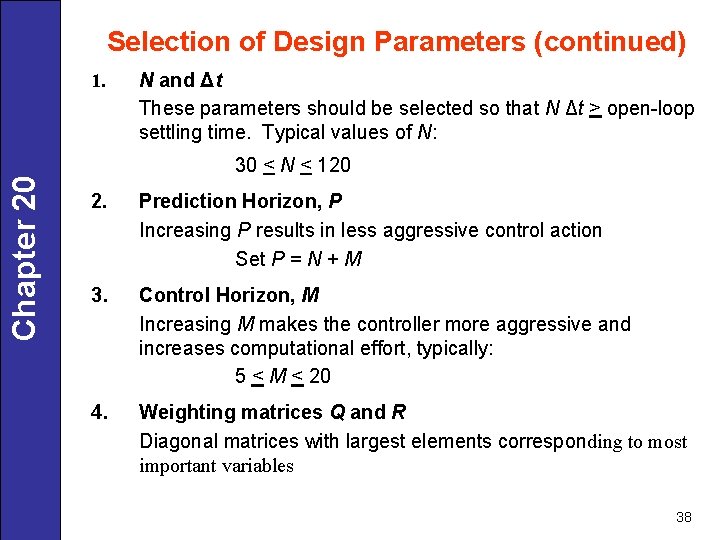
Selection of Design Parameters (continued) Chapter 20 1. N and Δt These parameters should be selected so that N Δt > open-loop settling time. Typical values of N: 30 < N < 120 2. Prediction Horizon, P Increasing P results in less aggressive control action Set P = N + M 3. Control Horizon, M Increasing M makes the controller more aggressive and increases computational effort, typically: 5 < M < 20 4. Weighting matrices Q and R Diagonal matrices with largest elements corresponding to most important variables 38

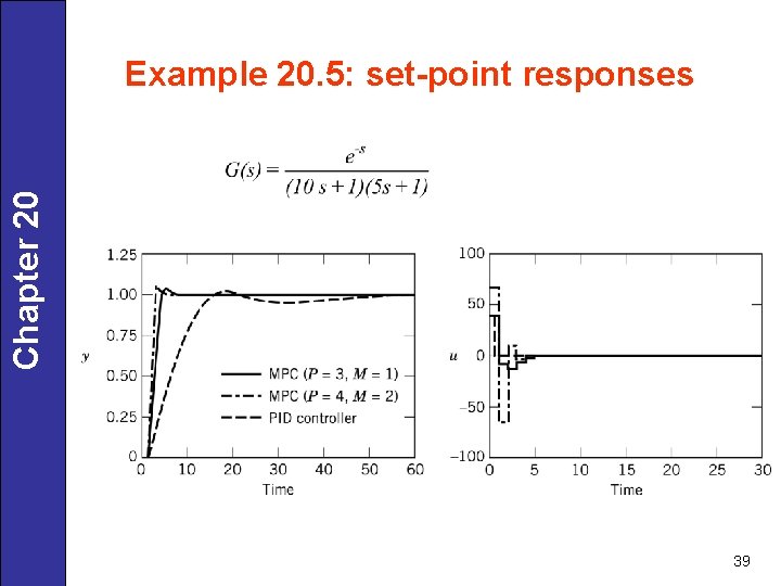
Chapter 20 Example 20. 5: set-point responses 39

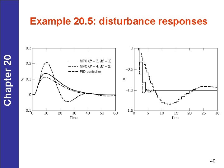
Chapter 20 Example 20. 5: disturbance responses 40