Chapter 2 An Introduction to Linear Programming Graphical

Chapter 2 An Introduction to Linear Programming : Graphical and Computer Methods Professor Ahmadi Slide 1

Learning Objectives n n n n Understand basic assumptions and properties of linear programming (LP) General LP notation LP formulation of the model A Maximization Problem Graphical solution A Minimization Problem Special Cases Formulating a Spreadsheet Model Slide 2

Introduction n Management decisions in many organizations involve trying to make most effective use of resources. • Include machinery, labor, money, time, warehouse space, and raw materials. • May be used to produce products - such as computers, automobiles, or clothing or • Provide services - such as package delivery, health services, or investment decisions. Slide 3

Mathematical Programming n Mathematical programming is used for resource allocation problems. n Linear programming (LP) is the most common type of mathematical programming. n One assumes that all the relevant input data and parameters are known with certainty in models (deterministic models). n Computers play an important role in the advancement and use of LP. Slide 4

Development of a LP Model n LP has been applied extensively to various problems areas - • medical, transportation, operations, petroleum • financial, marketing, accounting, • human resources, agriculture, and others n Development of all LP models can be examined in a three step process: • (1) formulation • (2) solution and • (3) interpretation. Slide 5

Properties of a LP Model 1. All problems seek to maximize or minimize some quantity, usually profit or cost (called the objective function). 2. LP models usually include restrictions, or constraints, that limit the degree to which one can pursue the objective. 3. There must be alternative courses of action from which one can choose. 4. The objective and constraints in LP problems must be expressed in terms of linear equations or inequalities. Slide 6

Three Steps of Developing LP Problem Formulation. • Process of translating problem scenario into a simple LP model framework with a set of mathematical relationships. Solution. • Mathematical relationships resulting from the formulation process are solved to identify an optimal solution. Interpretation and What-if Analysis. • Problem solver or analyst works with manager to u Interpret results and implications of problem solution. u Investigate changes in input parameters and model variables and impact on problem solution results. Slide 7

Basic Assumptions of a LP Model 1. Conditions of certainty exist. 2. Proportionality in the objective function and constraints (1 unit – 3 hours, 3 units 9 hours). 3. Additivity (the total of all activities equals the sum of the individual activities). 4. Divisibility assumption that solutions need not necessarily be in whole numbers (integers). Slide 8

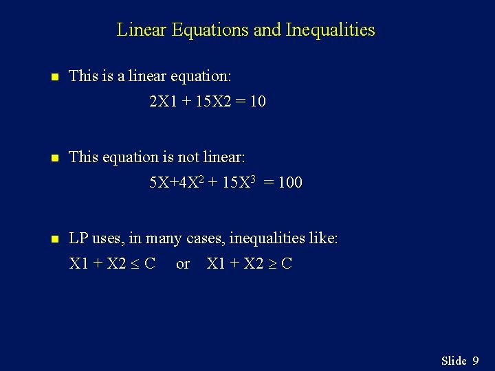
Linear Equations and Inequalities n This is a linear equation: 2 X 1 + 15 X 2 = 10 n This equation is not linear: 5 X+4 X 2 + 15 X 3 = 100 n LP uses, in many cases, inequalities like: X 1 + X 2 C or X 1 + X 2 C Slide 9

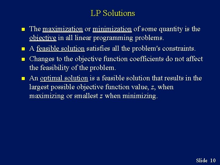
LP Solutions n n The maximization or minimization of some quantity is the objective in all linear programming problems. A feasible solution satisfies all the problem's constraints. Changes to the objective function coefficients do not affect the feasibility of the problem. An optimal solution is a feasible solution that results in the largest possible objective function value, z, when maximizing or smallest z when minimizing. Slide 10

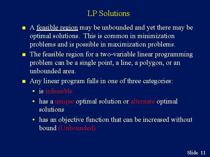
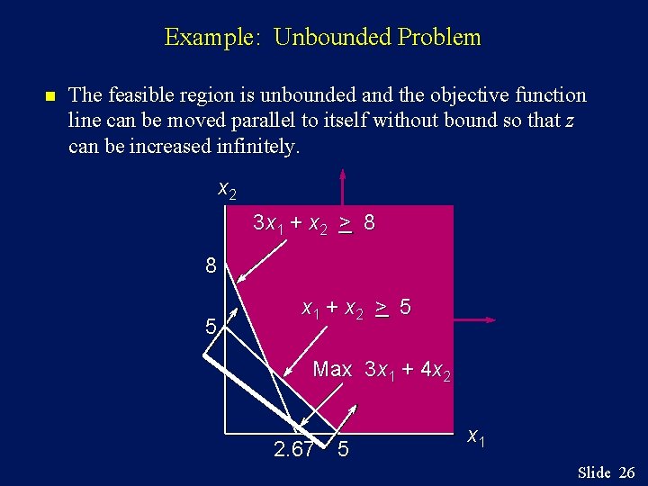
LP Solutions n n n A feasible region may be unbounded and yet there may be optimal solutions. This is common in minimization problems and is possible in maximization problems. The feasible region for a two-variable linear programming problem can be a single point, a line, a polygon, or an unbounded area. Any linear program falls in one of three categories: • is infeasible • has a unique optimal solution or alternate optimal solutions • has an objective function that can be increased without bound (Unbounded) Slide 11

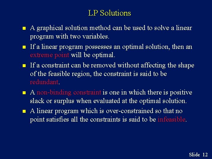
LP Solutions n n n A graphical solution method can be used to solve a linear program with two variables. If a linear program possesses an optimal solution, then an extreme point will be optimal. If a constraint can be removed without affecting the shape of the feasible region, the constraint is said to be redundant. A non-binding constraint is one in which there is positive slack or surplus when evaluated at the optimal solution. A linear program which is over-constrained so that no point satisfies all the constraints is said to be infeasible. Slide 12

Guidelines for Model Formulation n n Understand the problem thoroughly. Write a verbal statement of the objective function and each constraint. Define the decision variables. Write the objective function in terms of the decision variables. Write the constraints in terms of the decision variables. Slide 13

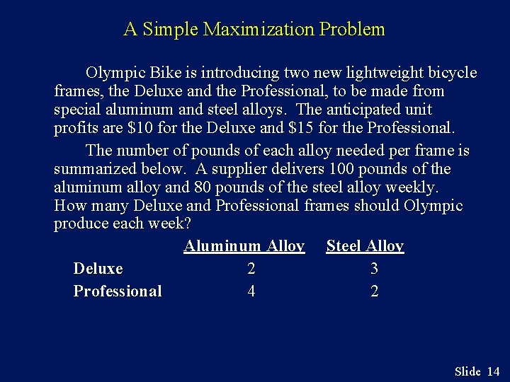
A Simple Maximization Problem Olympic Bike is introducing two new lightweight bicycle frames, the Deluxe and the Professional, to be made from special aluminum and steel alloys. The anticipated unit profits are $10 for the Deluxe and $15 for the Professional. The number of pounds of each alloy needed per frame is summarized below. A supplier delivers 100 pounds of the aluminum alloy and 80 pounds of the steel alloy weekly. How many Deluxe and Professional frames should Olympic produce each week? Aluminum Alloy Steel Alloy Deluxe 2 3 Professional 4 2 Slide 14

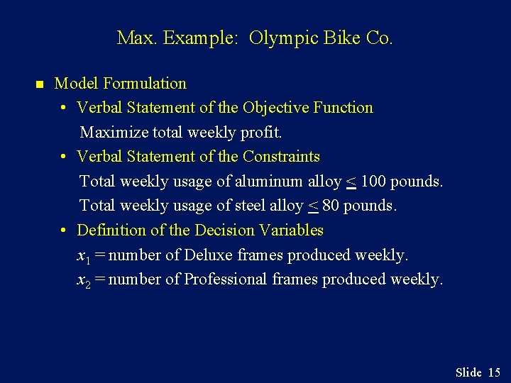
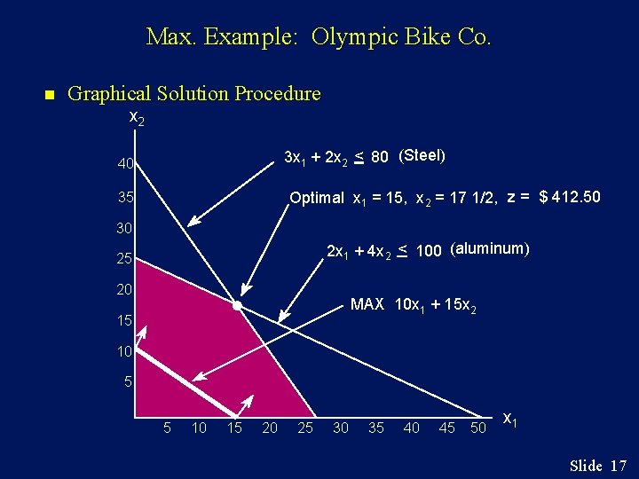
Max. Example: Olympic Bike Co. n Model Formulation • Verbal Statement of the Objective Function Maximize total weekly profit. • Verbal Statement of the Constraints Total weekly usage of aluminum alloy < 100 pounds. Total weekly usage of steel alloy < 80 pounds. • Definition of the Decision Variables x 1 = number of Deluxe frames produced weekly. x 2 = number of Professional frames produced weekly. Slide 15

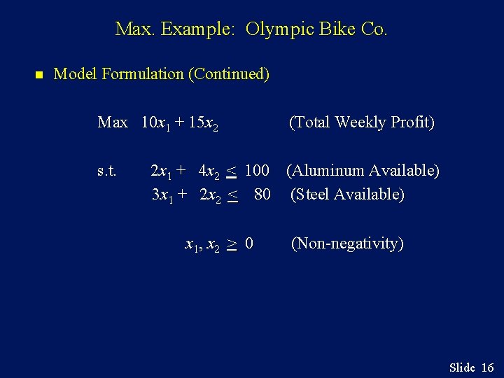
Max. Example: Olympic Bike Co. n Model Formulation (Continued) Max 10 x 1 + 15 x 2 s. t. (Total Weekly Profit) 2 x 1 + 4 x 2 < 100 (Aluminum Available) 3 x 1 + 2 x 2 < 80 (Steel Available) x 1, x 2 > 0 (Non-negativity) Slide 16

Max. Example: Olympic Bike Co. n Graphical Solution Procedure x 2 3 x 1 + 2 x 2 < 80 (Steel) 40 Optimal x 1 = 15, x 2 = 17 1/2, z = $ 412. 50 35 30 2 x 1 + 4 x 2 < 100 (aluminum) 25 20 MAX 10 x 1 + 15 x 2 15 10 5 5 10 15 20 25 30 35 40 45 50 x 1 Slide 17

Slack and Surplus Variables n n A linear program in which all the variables are nonnegative and all the constraints are equalities is said to be in standard form. Standard form is attained by adding slack variables to "less than or equal to" constraints, and by subtracting surplus variables from "greater than or equal to" constraints. Slack and surplus variables represent the difference between the left and right sides of the constraints. Slack and surplus variables have objective function coefficients equal to 0. Slide 18

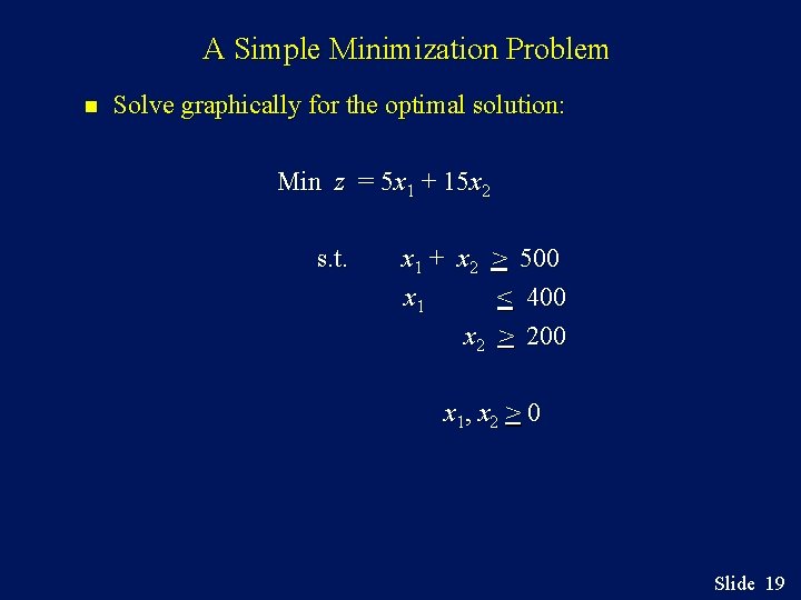
A Simple Minimization Problem n Solve graphically for the optimal solution: Min z = 5 x 1 + 15 x 2 s. t. x 1 + x 2 > 500 x 1 < 400 x 2 > 200 x 1, x 2 > 0 Slide 19

Special Cases n n n Alternative Optimal Solutions Infeasible Solutions Unbounded Problem Slide 20

Alternative Optimal Solutions n In the graphical method, if the objective function line is parallel to a boundary constraint in the direction of optimization, there alternate optimal solutions, with all points on this line segment being optimal. Example: Max z = 8 x 1 + 6 x 2 s. t. 4 x 1 + 3 x 2 < 12 9 x 1 + 12 x 2 < 36 x 1, x 2 > 0 Slide 21

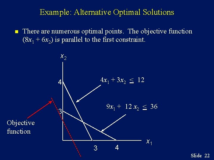
Example: Alternative Optimal Solutions n There are numerous optimal points. The objective function (8 x 1 + 6 x 2) is parallel to the first constraint. x 2 4 x 1 + 3 x 2 < 12 4 9 x 1 + 12 x 2 < 36 3 Objective function 3 4 x 1 Slide 22

Example: Infeasible Problem n Solve graphically for the optimal solution: Max z = 2 x 1 + 6 x 2 s. t. 4 x 1 + 3 x 2 < 12 2 x 1 + x 2 > 8 x 1, x 2 > 0 Slide 23

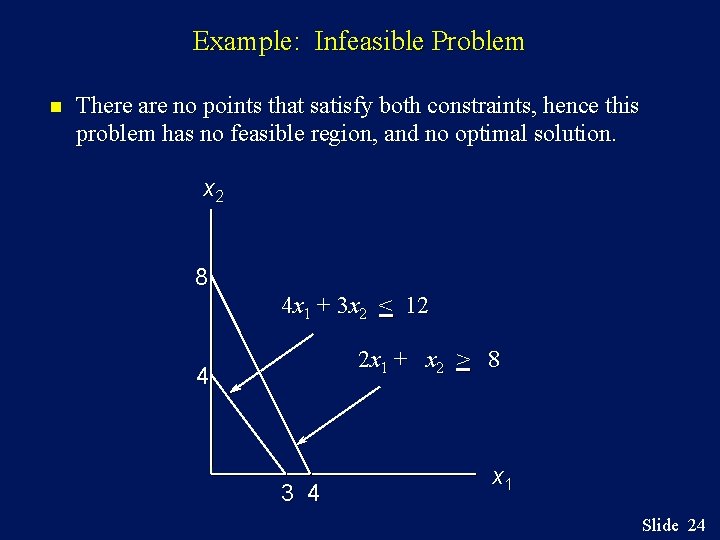
Example: Infeasible Problem n There are no points that satisfy both constraints, hence this problem has no feasible region, and no optimal solution. x 2 8 4 x 1 + 3 x 2 < 12 2 x 1 + x 2 > 8 4 3 4 x 1 Slide 24

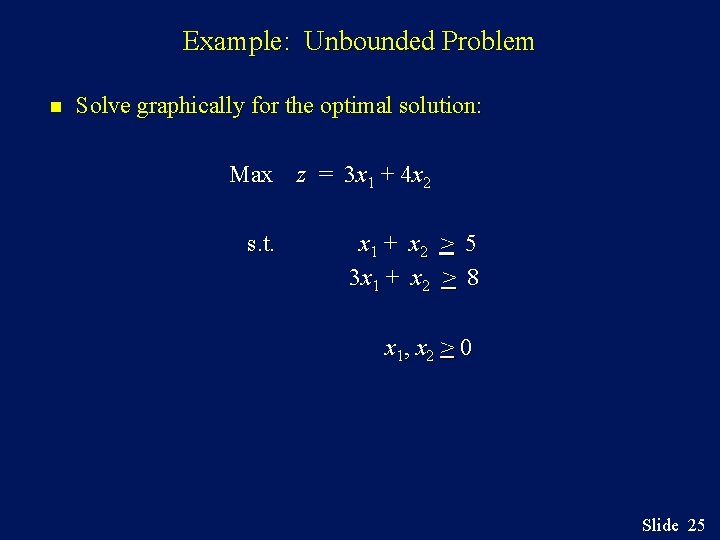
Example: Unbounded Problem n Solve graphically for the optimal solution: Max z = 3 x 1 + 4 x 2 s. t. x 1 + x 2 > 5 3 x 1 + x 2 > 8 x 1, x 2 > 0 Slide 25

Example: Unbounded Problem n The feasible region is unbounded and the objective function line can be moved parallel to itself without bound so that z can be increased infinitely. x 2 3 x 1 + x 2 > 8 8 5 x 1 + x 2 > 5 Max 3 x 1 + 4 x 2 2. 67 5 x 1 Slide 26

Using Excel for solving LP problems n Use “Solver” in Excel and solve the LP problems given previously. • Tools/Solver End of chapter 2 Slide 27