Chapter 10 Introduction to Simulation Modeling Introduction Simulation

Chapter 10 Introduction to Simulation Modeling

Introduction • Simulation model is a computer model that imitates a real-life situation. • It is like other mathematical models, but it explicitly incorporates uncertainty in one or more input variables. • When you run a simulation, you allow these random input variables to take on various values, and you keep track of any resulting output variables of interest. • In this way, you are able to see how the outputs vary as a function of the varying inputs. Winston/Albright Practical Management Science, 4 e South-Western/Cengage Learning © 2012 Thomson/South-Western 2007 ©

Introduction continued • The fundamental advantage of a simulation model is that it provides an entire distribution of results, not simply a single bottom-line result. • Each different set of values for the uncertain quantities can be considered a scenario. • Simulation allows the company to generate many scenarios, each leading to a particular NPV. • In the end, it sees a whole distribution of NPVs, not a single best guess. The company can see what the NPV will be on average, and it can also see worst-case and best-case results. Winston/Albright Practical Management Science, 4 e South-Western/Cengage Learning © 2012 Thomson/South-Western 2007 ©

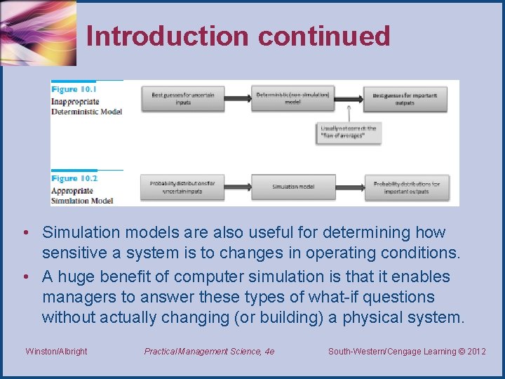
Introduction continued • These approaches are summarized in the two figures on the next slide. • First figure indicates that the deterministic (non-simulation) approach, using best guesses for the uncertain inputs, is generally not the appropriate method. – It leads to the “flaw of averages, ” as we will discuss later in the chapter. – The problem is that the outputs from the deterministic model are often not representative of the true outputs. • The appropriate method is shown second. – Here the uncertainty is modeled explicitly with random inputs, and the end result is a probability distribution for each of the important outputs. Winston/Albright Practical Management Science, 4 e South-Western/Cengage Learning © 2012 Thomson/South-Western 2007 ©

Introduction continued • Simulation models are also useful for determining how sensitive a system is to changes in operating conditions. • A huge benefit of computer simulation is that it enables managers to answer these types of what-if questions without actually changing (or building) a physical system. Winston/Albright Practical Management Science, 4 e South-Western/Cengage Learning © 2012 Thomson/South-Western 2007 ©

Introduction continued • Spreadsheet simulation modeling is quite similar to the other modeling applications in this book. – You begin with input variables and then relate these with appropriate Excel formulas to produce output variables of interest. – The main difference is that simulation uses random numbers to drive the whole process. These random numbers are generated with special functions that we will discuss in detail. – Each time the spreadsheet recalculates, all of the random numbers change. – This provides the ability to model the logical process once and then use Excel’s recalculation ability to generate many different scenarios. Winston/Albright Practical Management Science, 4 e South-Western/Cengage Learning © 2012 Thomson/South-Western 2007 ©

Probability distributions for input variables • The primary difference between the spreadsheet models you have developed so far and simulation models is that at least one of the input variable cells in a simulation model contains random numbers. • Each time the spreadsheet recalculates, the random numbers change, and the new random values of the inputs produce new values of the outputs. This is the essence of simulation—it enables you to see how outputs vary as random inputs change. Winston/Albright Practical Management Science, 4 e South-Western/Cengage Learning © 2012 Thomson/South-Western 2007 ©

Types of probability distributions • We begin by adding a few useful probability distributions to this toolbox. • However, before adding any specific distributions, it is useful to provide a brief review of some important general characteristics of probability distributions. These include the following distinctions: – – Discrete versus continuous Symmetric versus skewed Bounded versus unbounded Nonnegative versus unrestricted. Winston/Albright Practical Management Science, 4 e South-Western/Cengage Learning © 2012 Thomson/South-Western 2007 ©

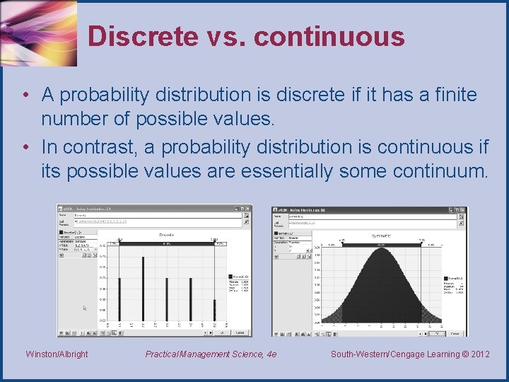
Discrete vs. continuous • A probability distribution is discrete if it has a finite number of possible values. • In contrast, a probability distribution is continuous if its possible values are essentially some continuum. Winston/Albright Practical Management Science, 4 e South-Western/Cengage Learning © 2012 Thomson/South-Western 2007 ©

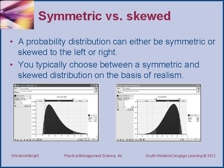
Symmetric vs. skewed • A probability distribution can either be symmetric or skewed to the left or right. • You typically choose between a symmetric and skewed distribution on the basis of realism. Winston/Albright Practical Management Science, 4 e South-Western/Cengage Learning © 2012 Thomson/South-Western 2007 ©

Bounded vs. unbounded • A probability distribution is bounded if there are values A and B such that no possible value can be less than A or greater than B. The value A is then the minimum possible value, and the value B is the maximum possible value. • The distribution is unbounded if there are no such bounds. – Actually, it is possible for a distribution to be bounded in one direction but not the other. Winston/Albright Practical Management Science, 4 e South-Western/Cengage Learning © 2012 Thomson/South-Western 2007 ©

Nonnegative vs. unrestricted • One important special case of bounded distributions is when the only possible values are nonnegative. • For example, if you want to model the random cost of manufacturing a new product, you know for sure that this cost must be nonnegative. • There are many other such examples. In such cases, you should model the randomness with a probability distribution that is bounded below by 0. This rules out negative values that make no practical sense. Winston/Albright Practical Management Science, 4 e South-Western/Cengage Learning © 2012 Thomson/South-Western 2007 ©

Common probability distributions • Now that you know the types of probability distributions available, you can add some common probability distributions to your toolbox. • The file Probability Distributions. xlsx was developed to help you learn and explore these. • Each sheet in this file illustrates a particular probability distribution. • It is important to realize that each of the following distributions is really a family of distributions. • Each member of the family is specified by one or more parameters. Winston/Albright Practical Management Science, 4 e South-Western/Cengage Learning © 2012 Thomson/South-Western 2007 ©

Simulation and the flaw of averages • To help motivate simulation modeling in general, we present a simple example in this section. • It will clearly show the distinction between a deterministic model with best-guess inputs and an appropriate simulation model. • In doing so, it will illustrate a pitfall called the “flaw of averages” that you should always try to avoid. • This concept is demonstrated in Example 10. 1 Winston/Albright Practical Management Science, 4 e South-Western/Cengage Learning © 2012 Thomson/South-Western 2007 ©

Simulation with built-in Excel tools • In this section, we show spreadsheet simulation models can be developed analyzed with Excel’s built-in tools without using add-ins. • To illustrate the Excel-only procedure, we continue analyzing the calendar problem from Example 10. 1. This general problem occurs when a company (such as a news vendor) must make a one-time purchase of a product (such as a newspaper) to meet customer demands for a certain period of time. • Winston/Albright Example 10. 2 is typical. Practical Management Science, 4 e South-Western/Cengage Learning © 2012 Thomson/South-Western 2007 ©

@RISK models with a single random input variable • In the remainder of this section we illustrate some of @RISK’s functionality by revisiting the Walton Bookstore example. • The development of a simulation model is basically a two-step procedure. – The first step is to build the model itself. This step requires you to enter all of the logic that transforms inputs (including @RISK functions such as RISKDISCRETE) into outputs (such as profit). – However, once this logic has been incorporated, @RISK takes over in the second step. Winston/Albright Practical Management Science, 4 e South-Western/Cengage Learning © 2012 Thomson/South-Western 2007 ©

@RISK models with several random input variables • We conclude this section with another modification of the Walton Bookstore example. • To this point, there has been a single random variable, demand. • Often there are several random variables, each reflecting some uncertainty, and you want to include each of these in the simulation model. • The following example illustrates how this can be done, and it also illustrates a very useful feature of @RISK, its sensitivity analysis. Winston/Albright Practical Management Science, 4 e South-Western/Cengage Learning © 2012 Thomson/South-Western 2007 ©

The effects of input distributions on results • The randomness in input variables causes the variability in the output variables. We now briefly explore whether the choice of input distribution(s) makes much difference in the distribution of an output variable such as profit. • This is an important question. If the choice of input distributions doesn’t matter much, then you do not need to agonize over this choice. • However, if it does make a difference, then you have to be more careful about choosing the most appropriate input distribution for any particular situation. Unfortunately, it is impossible to answer the question definitively. Winston/Albright Practical Management Science, 4 e South-Western/Cengage Learning © 2012 Thomson/South-Western 2007 ©

The effects of input distributions on results continued • We discuss two types of sensitivity analysis in this section. First, we check whether the shape of the input distribution matters. In the Walton Bookstore example, we assumed a triangularly distributed demand with some skewness. • Are the results basically the same if a symmetric distribution such as the normal distribution is used instead? Winston/Albright Practical Management Science, 4 e South-Western/Cengage Learning © 2012 Thomson/South-Western 2007 ©

The effects of input distributions on results continued • Second, we check whether the independence of input variables that have been assumed implicitly to this point is crucial to the output results. Many random quantities in real situations are not independent; they are positively or negatively correlated. • Fortunately, @RISK enables you to build correlation into a model. We analyze the effect of this correlation. • Example 10. 5 demonstrates this concept. Winston/Albright Practical Management Science, 4 e South-Western/Cengage Learning © 2012 Thomson/South-Western 2007 ©

Effects of correlated input variables • Until now, all of the random numbers generated with @RISK functions have been probabilistically independent. • This means, for example, that if a random value in one cell is much larger than its mean, the random values in other cells are completely unaffected. • They are no more likely to be abnormally large or small than if the first value had been average or below average. Sometimes, however, independence is unrealistic. In such cases, the random numbers should be correlated in some way. Winston/Albright Practical Management Science, 4 e South-Western/Cengage Learning © 2012 Thomson/South-Western 2007 ©

Effects of correlated input variables • As an example, you might expect daily stock price changes for two companies in the same industry to be positively correlated. • If the price of one oil company increases, you might expect the price of another oil company to increase as well. • @RISK enables you to build in this correlated behavior with the RISKCORRMAT function, as we illustrate in the continuation of the Walton example. Winston/Albright Practical Management Science, 4 e South-Western/Cengage Learning © 2012 Thomson/South-Western 2007 ©

Conclusion • Simulation has traditionally not received the attention it deserves in management science courses. • The primary reason for this has been the lack of easy-to-use simulation software. • Now, with Excel’s built-in simulation capabilities, plus powerful and affordable add-ins such as @RISK, simulation is receiving its rightful emphasis. Winston/Albright Practical Management Science, 4 e South-Western/Cengage Learning © 2012 Thomson/South-Western 2007 ©

Conclusion continued • The world is full of uncertainty, which is what makes simulation so valuable. • Simulation models provide important insights that are missing in models that do not incorporate uncertainty explicitly. • In addition, simulation models are relatively easy to understand develop. Therefore, we suspect that simulation models (together with optimization models) will soon be the primary emphasis of • many management science courses—if they are not already. Winston/Albright Practical Management Science, 4 e South-Western/Cengage Learning © 2012 Thomson/South-Western 2007 ©

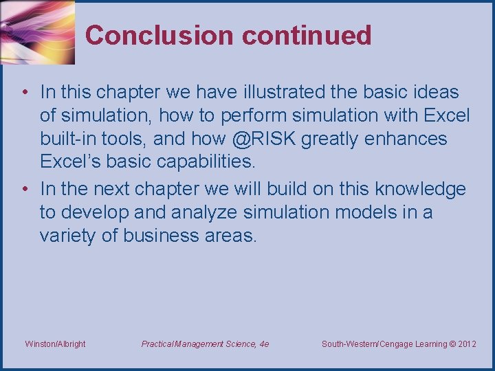
Conclusion continued • In this chapter we have illustrated the basic ideas of simulation, how to perform simulation with Excel built-in tools, and how @RISK greatly enhances Excel’s basic capabilities. • In the next chapter we will build on this knowledge to develop and analyze simulation models in a variety of business areas. Winston/Albright Practical Management Science, 4 e South-Western/Cengage Learning © 2012 Thomson/South-Western 2007 ©

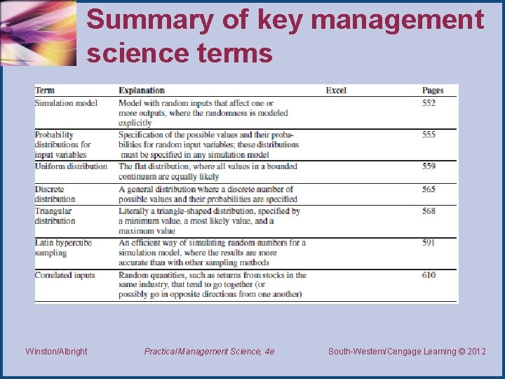
Summary of key management science terms Winston/Albright Practical Management Science, 4 e South-Western/Cengage Learning © 2012 Thomson/South-Western 2007 ©

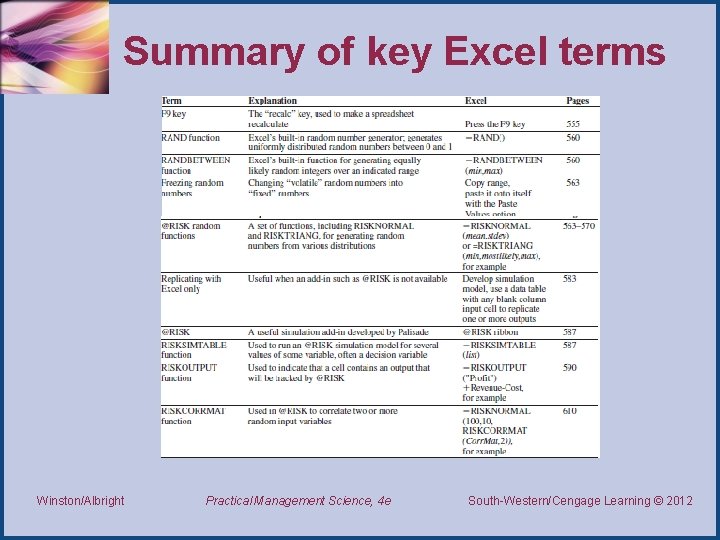
Summary of key Excel terms Winston/Albright Practical Management Science, 4 e South-Western/Cengage Learning © 2012 Thomson/South-Western 2007 ©

End of Chapter 10