Chapter 2 Modeling Complex Systems Simulation Modeling and
- Slides: 38

Chapter 2 Modeling Complex Systems Simulation Modeling and Analysis – Chapter 2 – Modeling Complex Systems 1

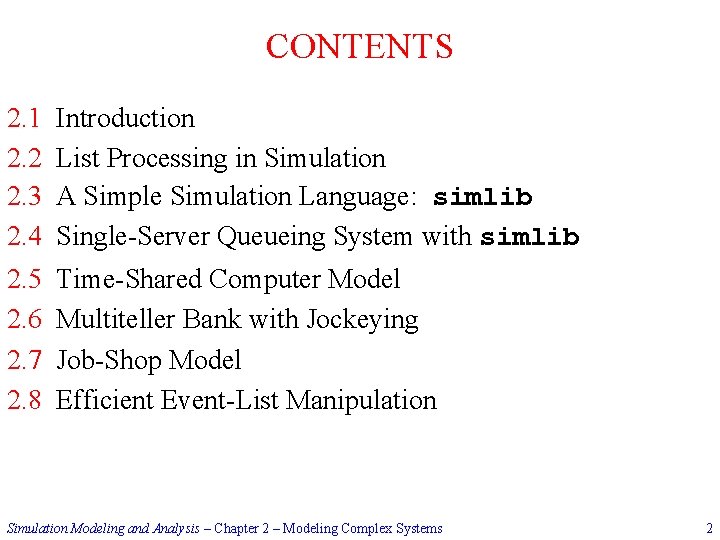
CONTENTS 2. 1 2. 2 2. 3 2. 4 Introduction List Processing in Simulation A Simple Simulation Language: simlib Single-Server Queueing System with simlib 2. 5 2. 6 2. 7 2. 8 Time-Shared Computer Model Multiteller Bank with Jockeying Job-Shop Model Efficient Event-List Manipulation Simulation Modeling and Analysis – Chapter 2 – Modeling Complex Systems 2

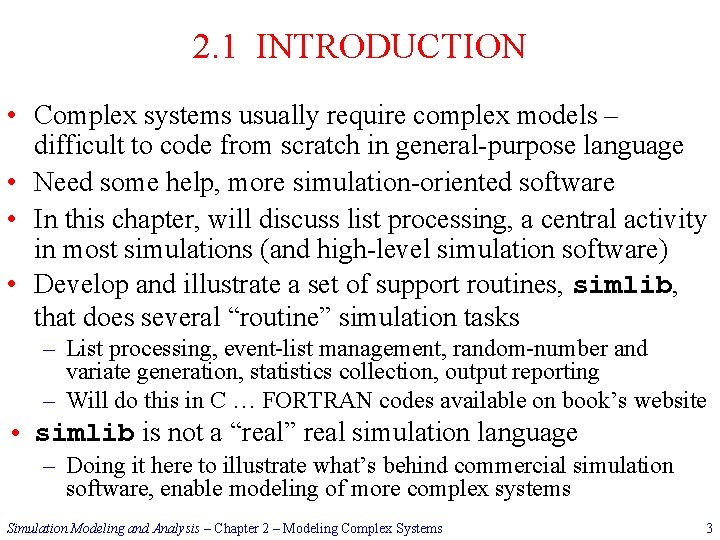
2. 1 INTRODUCTION • Complex systems usually require complex models – difficult to code from scratch in general-purpose language • Need some help, more simulation-oriented software • In this chapter, will discuss list processing, a central activity in most simulations (and high-level simulation software) • Develop and illustrate a set of support routines, simlib, that does several “routine” simulation tasks – List processing, event-list management, random-number and variate generation, statistics collection, output reporting – Will do this in C … FORTRAN codes available on book’s website • simlib is not a “real” real simulation language – Doing it here to illustrate what’s behind commercial simulation software, enable modeling of more complex systems Simulation Modeling and Analysis – Chapter 2 – Modeling Complex Systems 3

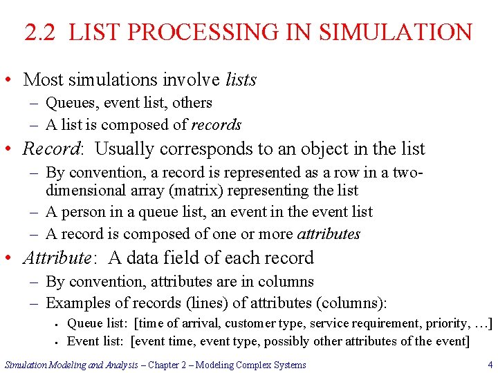
2. 2 LIST PROCESSING IN SIMULATION • Most simulations involve lists – Queues, event list, others – A list is composed of records • Record: Usually corresponds to an object in the list – By convention, a record is represented as a row in a twodimensional array (matrix) representing the list – A person in a queue list, an event in the event list – A record is composed of one or more attributes • Attribute: A data field of each record – By convention, attributes are in columns – Examples of records (lines) of attributes (columns): § § Queue list: [time of arrival, customer type, service requirement, priority, …] Event list: [event time, event type, possibly other attributes of the event] Simulation Modeling and Analysis – Chapter 2 – Modeling Complex Systems 4

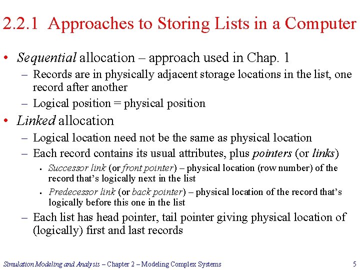
2. 2. 1 Approaches to Storing Lists in a Computer • Sequential allocation – approach used in Chap. 1 – Records are in physically adjacent storage locations in the list, one record after another – Logical position = physical position • Linked allocation – Logical location need not be the same as physical location – Each record contains its usual attributes, plus pointers (or links) § § Successor link (or front pointer) – physical location (row number) of the record that’s logically next in the list Predecessor link (or back pointer) – physical location of the record that’s logically before this one in the list – Each list has head pointer, tail pointer giving physical location of (logically) first and last records Simulation Modeling and Analysis – Chapter 2 – Modeling Complex Systems 5

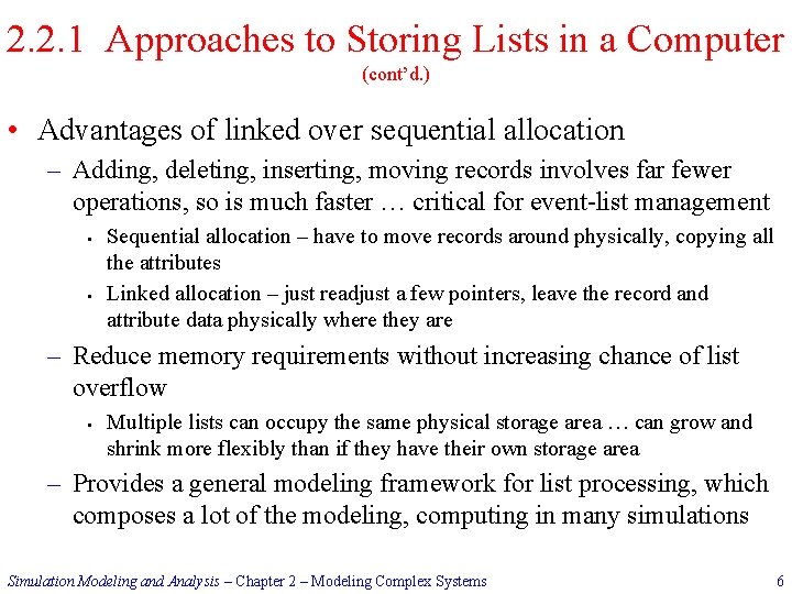
2. 2. 1 Approaches to Storing Lists in a Computer (cont’d. ) • Advantages of linked over sequential allocation – Adding, deleting, inserting, moving records involves far fewer operations, so is much faster … critical for event-list management § § Sequential allocation – have to move records around physically, copying all the attributes Linked allocation – just readjust a few pointers, leave the record and attribute data physically where they are – Reduce memory requirements without increasing chance of list overflow § Multiple lists can occupy the same physical storage area … can grow and shrink more flexibly than if they have their own storage area – Provides a general modeling framework for list processing, which composes a lot of the modeling, computing in many simulations Simulation Modeling and Analysis – Chapter 2 – Modeling Complex Systems 6

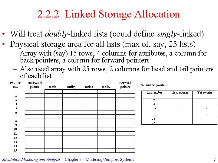
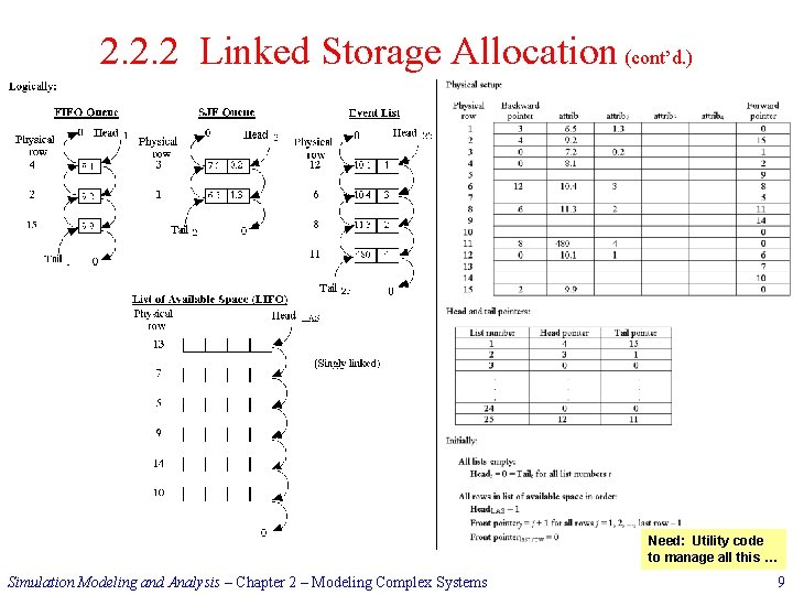
2. 2. 2 Linked Storage Allocation • Will treat doubly-linked lists (could define singly-linked) • Physical storage area for all lists (max of, say, 25 lists) – Array with (say) 15 rows, 4 columns for attributes, a column for back pointers, a column forward pointers – Also need array with 25 rows, 2 columns for head and tail pointers of each list Simulation Modeling and Analysis – Chapter 2 – Modeling Complex Systems 7

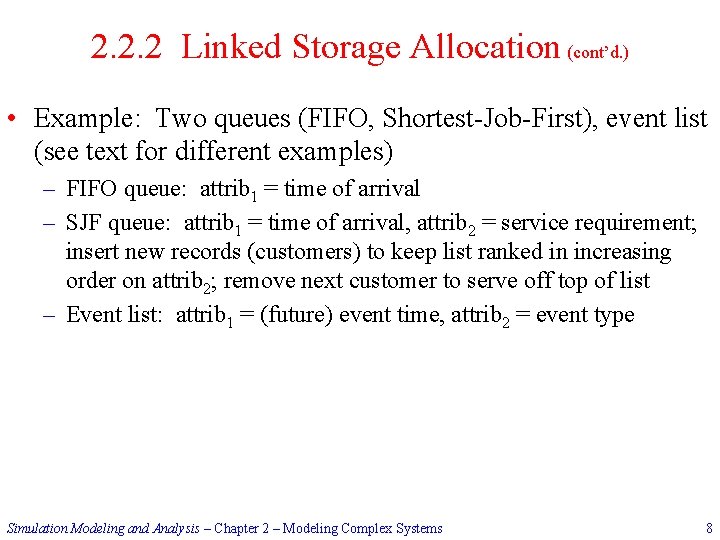
2. 2. 2 Linked Storage Allocation (cont’d. ) • Example: Two queues (FIFO, Shortest-Job-First), event list (see text for different examples) – FIFO queue: attrib 1 = time of arrival – SJF queue: attrib 1 = time of arrival, attrib 2 = service requirement; insert new records (customers) to keep list ranked in increasing order on attrib 2; remove next customer to serve off top of list – Event list: attrib 1 = (future) event time, attrib 2 = event type Simulation Modeling and Analysis – Chapter 2 – Modeling Complex Systems 8

2. 2. 2 Linked Storage Allocation (cont’d. ) Need: Utility code to manage all this … Simulation Modeling and Analysis – Chapter 2 – Modeling Complex Systems 9

2. 3 A SIMPLE SIMULATION LANGUAGE: simlib • Some C functions – rudimentary simulation “language” – Source code in Appendix 2 A, and on book’s website – Also available in “legacy” FORTRAN on book’s website • Capabilities – – – List processing (pointers, file a record, remove a record) Processes event list Tallies statistical counters Generate random numbers, variates from some distributions Provide “standard” output (optional) • Not a “real” simulation language – incomplete, inefficient – But illustrates what’s in real simulation software, how it works Simulation Modeling and Analysis – Chapter 2 – Modeling Complex Systems 10

2. 3 A Simple Simulation Language: simlib (cont’d. ) • Heart of simlib is a collection of doubly linked lists – All live together in dynamic memory – space allocated as new records are filed in lists, freed when records are removed from lists – Maximum of 25 lists – Records in lists can have a maximum of 10 attributes – Data are stored as type float – Uses dynamic storage allocation, so total number of records in all lists is limited only by hardware – List 25 always reserved for event list § § § Always: attribute 1 = (future) event time, attribute 2 = event type attributes 3 -10 can be used for other event attributes Kept sorted in increasing order on event time – next event is always on top • User must #include simlib. h for required declarations, definitions – simlib. h in turn #includes simlibdefs. h Simulation Modeling and Analysis – Chapter 2 – Modeling Complex Systems 11

2. 3 A Simple Simulation Language: simlib (cont’d. ) • Key simlib variables and constants sim_time = simulation clock; updated by simlib next_event_type = type of next event; determined by simlib transfer[i]: float array indexed on i = 1, 2, …, 10 for transferring attributes of records into and out of lists maxatr = max number of attributes in any list; defaults to 10, but user can initialize to < 10 for improved efficiency (cannot be set to < 4 due to the way simlib works) list_size[list] = current number of records in list; maintained by simlib list_rank[list] = attribute number (if any) on which list is to be ranked (incr. or decr. ); must be initialized by user FIRST, LAST, INCREASING, DECREASING: symbolic constants for options of filing a record into a list LIST_EVENT, EVENT_TIME, EVENT_TYPE: symbolic constants for event-list number, attribute number of event time, attribute number of event type Simulation Modeling and Analysis – Chapter 2 – Modeling Complex Systems 12

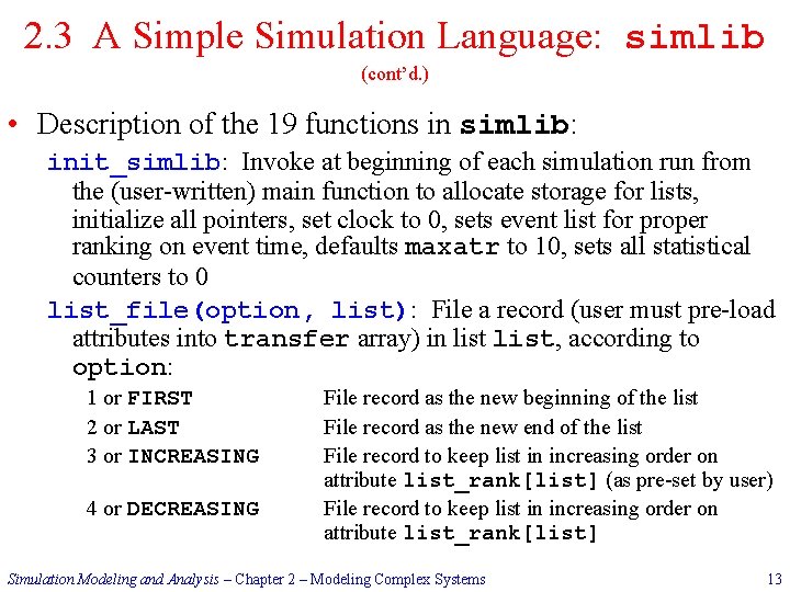
2. 3 A Simple Simulation Language: simlib (cont’d. ) • Description of the 19 functions in simlib: init_simlib: Invoke at beginning of each simulation run from the (user-written) main function to allocate storage for lists, initialize all pointers, set clock to 0, sets event list for proper ranking on event time, defaults maxatr to 10, sets all statistical counters to 0 list_file(option, list): File a record (user must pre-load attributes into transfer array) in list, according to option: 1 or FIRST 2 or LAST 3 or INCREASING 4 or DECREASING File record as the new beginning of the list File record as the new end of the list File record to keep list in increasing order on attribute list_rank[list] (as pre-set by user) File record to keep list in increasing order on attribute list_rank[list] Simulation Modeling and Analysis – Chapter 2 – Modeling Complex Systems 13

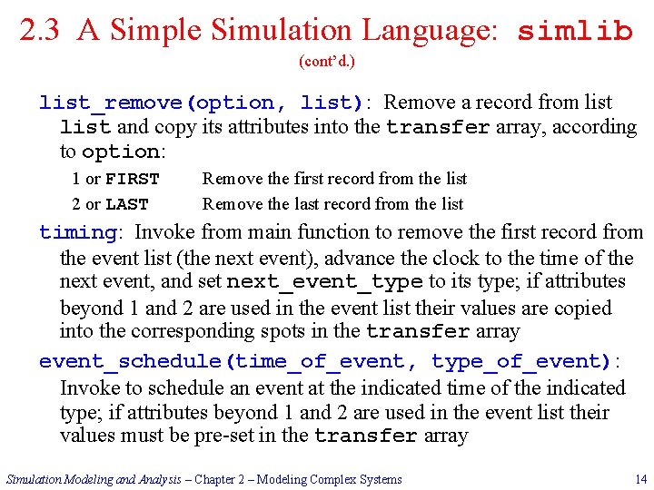
2. 3 A Simple Simulation Language: simlib (cont’d. ) list_remove(option, list): Remove a record from list and copy its attributes into the transfer array, according to option: 1 or FIRST 2 or LAST Remove the first record from the list Remove the last record from the list timing: Invoke from main function to remove the first record from the event list (the next event), advance the clock to the time of the next event, and set next_event_type to its type; if attributes beyond 1 and 2 are used in the event list their values are copied into the corresponding spots in the transfer array event_schedule(time_of_event, type_of_event): Invoke to schedule an event at the indicated time of the indicated type; if attributes beyond 1 and 2 are used in the event list their values must be pre-set in the transfer array Simulation Modeling and Analysis – Chapter 2 – Modeling Complex Systems 14

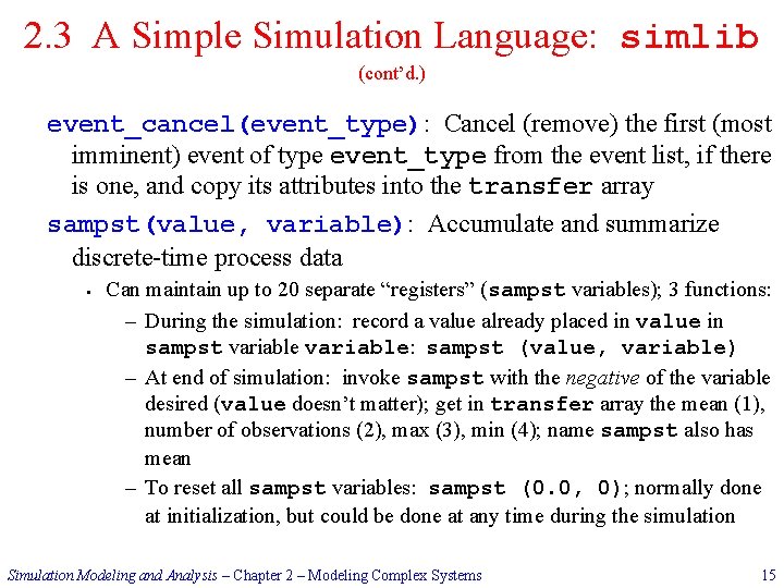
2. 3 A Simple Simulation Language: simlib (cont’d. ) event_cancel(event_type): Cancel (remove) the first (most imminent) event of type event_type from the event list, if there is one, and copy its attributes into the transfer array sampst(value, variable): Accumulate and summarize discrete-time process data § Can maintain up to 20 separate “registers” (sampst variables); 3 functions: – During the simulation: record a value already placed in value in sampst variable: sampst (value, variable) – At end of simulation: invoke sampst with the negative of the variable desired (value doesn’t matter); get in transfer array the mean (1), number of observations (2), max (3), min (4); name sampst also has mean – To reset all sampst variables: sampst (0. 0, 0); normally done at initialization, but could be done at any time during the simulation Simulation Modeling and Analysis – Chapter 2 – Modeling Complex Systems 15

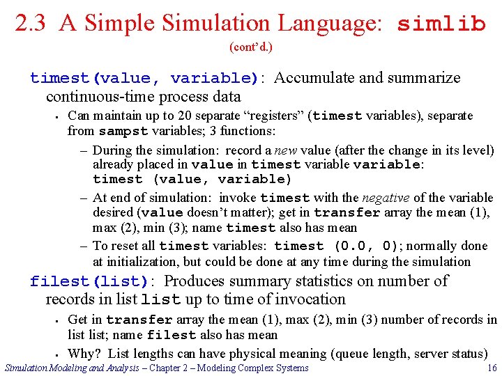
2. 3 A Simple Simulation Language: simlib (cont’d. ) timest(value, variable): Accumulate and summarize continuous-time process data § Can maintain up to 20 separate “registers” (timest variables), separate from sampst variables; 3 functions: – During the simulation: record a new value (after the change in its level) already placed in value in timest variable: timest (value, variable) – At end of simulation: invoke timest with the negative of the variable desired (value doesn’t matter); get in transfer array the mean (1), max (2), min (3); name timest also has mean – To reset all timest variables: timest (0. 0, 0); normally done at initialization, but could be done at any time during the simulation filest(list): Produces summary statistics on number of records in list up to time of invocation § § Get in transfer array the mean (1), max (2), min (3) number of records in list; name filest also has mean Why? List lengths can have physical meaning (queue length, server status) Simulation Modeling and Analysis – Chapter 2 – Modeling Complex Systems 16

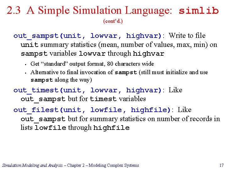
2. 3 A Simple Simulation Language: simlib (cont’d. ) out_sampst(unit, lowvar, highvar): Write to file unit summary statistics (mean, number of values, max, min) on sampst variables lowvar through highvar § § Get “standard” output format, 80 characters wide Alternative to final invocation of sampst (still must initialize and use sampst along the way) out_timest(unit, lowvar, highvar): Like out_sampst but for timest variables out_filest(unit, lowfile, highfile): Like out_sampst but for summary statistics on number of records in lists lowfile through highfile Simulation Modeling and Analysis – Chapter 2 – Modeling Complex Systems 17

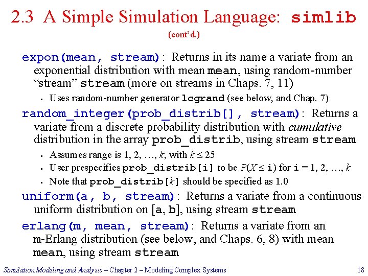
2. 3 A Simple Simulation Language: simlib (cont’d. ) expon(mean, stream): Returns in its name a variate from an exponential distribution with mean, using random-number “stream” stream (more on streams in Chaps. 7, 11) § Uses random-number generator lcgrand (see below, and Chap. 7) random_integer(prob_distrib[], stream): Returns a variate from a discrete probability distribution with cumulative distribution in the array prob_distrib, using stream § § § Assumes range is 1, 2, …, k, with k 25 User prespecifies prob_distrib[i] to be P(X i) for i = 1, 2, …, k Note that prob_distrib[k] should be specified as 1. 0 uniform(a, b, stream): Returns a variate from a continuous uniform distribution on [a, b], using stream erlang(m, mean, stream): Returns a variate from an m-Erlang distribution (see below, and Chaps. 6, 8) with mean, using stream Simulation Modeling and Analysis – Chapter 2 – Modeling Complex Systems 18

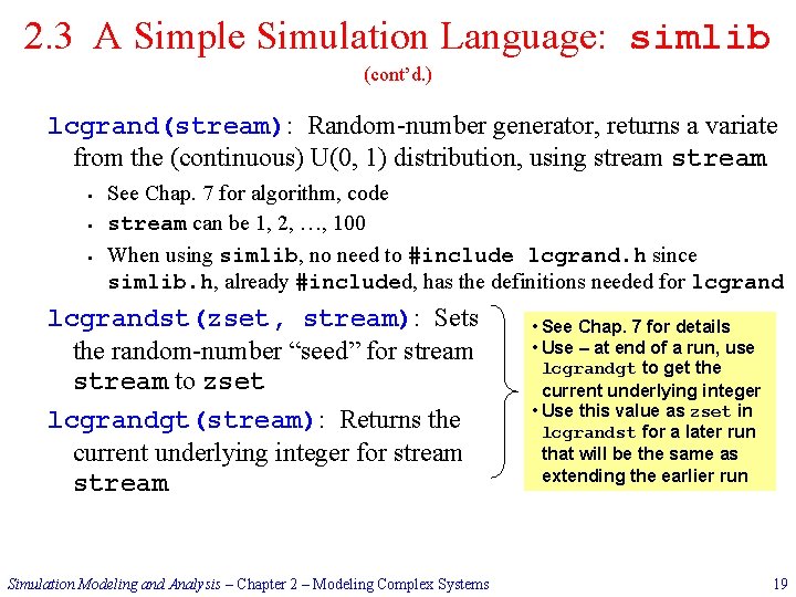
2. 3 A Simple Simulation Language: simlib (cont’d. ) lcgrand(stream): Random-number generator, returns a variate from the (continuous) U(0, 1) distribution, using stream § § § See Chap. 7 for algorithm, code stream can be 1, 2, …, 100 When using simlib, no need to #include lcgrand. h since simlib. h, already #included, has the definitions needed for lcgrandst(zset, stream): Sets the random-number “seed” for stream to zset lcgrandgt(stream): Returns the current underlying integer for stream Simulation Modeling and Analysis – Chapter 2 – Modeling Complex Systems • See Chap. 7 for details • Use – at end of a run, use lcgrandgt to get the current underlying integer • Use this value as zset in lcgrandst for a later run that will be the same as extending the earlier run 19

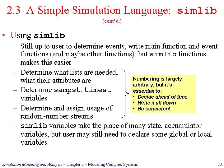
2. 3 A Simple Simulation Language: simlib (cont’d. ) • Using simlib – Still up to user to determine events, write main function and event functions (and maybe other functions), but simlib functions makes this easier – Determine what lists are needed, Numbering is largely what their attributes are arbitrary, but it’s – Determine sampst, timest essential to: • Decide ahead of time variables • Write it all down • Be consistent – Determine and assign usage of random-number streams – simlib variables take the place of many state, accumulator variables, but user may still need to declare some global or local variables Simulation Modeling and Analysis – Chapter 2 – Modeling Complex Systems 20

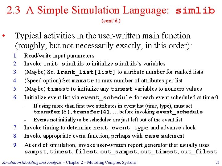
2. 3 A Simple Simulation Language: simlib (cont’d. ) • Typical activities in the user-written main function (roughly, but not necessarily exactly, in this order): 1. 2. 3. 4. 5. 6. Read/write input parameters Invoke init_simlib to initialize simlib’s variables (Maybe) Set lrank_list[list] to attribute number for ranked lists (Speed option) Set maxatr to max number of attributes per list (Maybe) timest to initialize any timest variables to nonzero values Initialize event list via event_schedule for each event scheduled at time 0 – – 7. 8. 9. If using more than first two attributes in event list (time, type), must set transfer[3], transfer[4], … before invoking event_schedule Events not initially to be scheduled are just left out of the event list Invoke timing to determine next_event_type and advance clock Invoke appropriate event function, perhaps with case statement At end of simulation, invoke user-written report generator that usually uses sampst, timest, filest, out_sampst, out_timest, out_filest Simulation Modeling and Analysis – Chapter 2 – Modeling Complex Systems 21

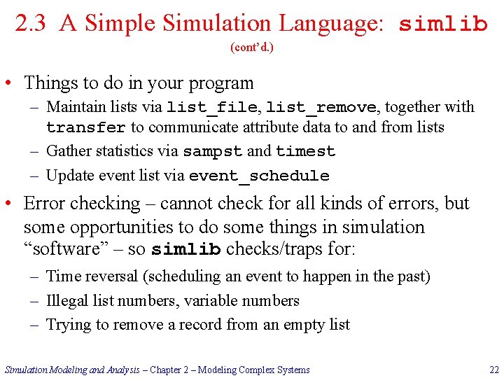
2. 3 A Simple Simulation Language: simlib (cont’d. ) • Things to do in your program – Maintain lists via list_file, list_remove, together with transfer to communicate attribute data to and from lists – Gather statistics via sampst and timest – Update event list via event_schedule • Error checking – cannot check for all kinds of errors, but some opportunities to do some things in simulation “software” – so simlib checks/traps for: – Time reversal (scheduling an event to happen in the past) – Illegal list numbers, variable numbers – Trying to remove a record from an empty list Simulation Modeling and Analysis – Chapter 2 – Modeling Complex Systems 22

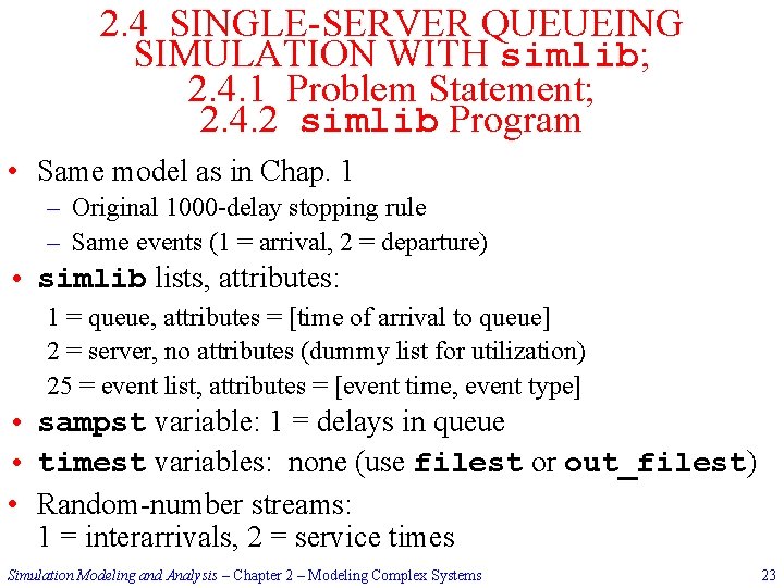
2. 4 SINGLE-SERVER QUEUEING SIMULATION WITH simlib; 2. 4. 1 Problem Statement; 2. 4. 2 simlib Program • Same model as in Chap. 1 – Original 1000 -delay stopping rule – Same events (1 = arrival, 2 = departure) • simlib lists, attributes: 1 = queue, attributes = [time of arrival to queue] 2 = server, no attributes (dummy list for utilization) 25 = event list, attributes = [event time, event type] • sampst variable: 1 = delays in queue • timest variables: none (use filest or out_filest) • Random-number streams: 1 = interarrivals, 2 = service times Simulation Modeling and Analysis – Chapter 2 – Modeling Complex Systems 23

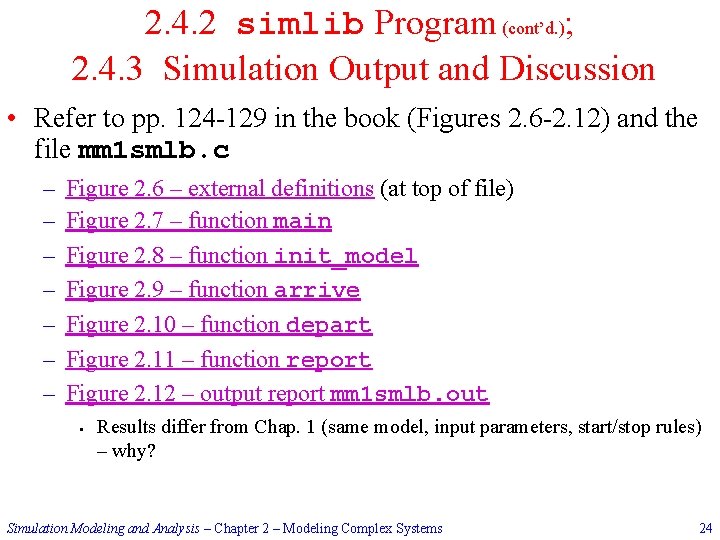
2. 4. 2 simlib Program (cont’d. ); 2. 4. 3 Simulation Output and Discussion • Refer to pp. 124 -129 in the book (Figures 2. 6 -2. 12) and the file mm 1 smlb. c – – – – Figure 2. 6 – external definitions (at top of file) Figure 2. 7 – function main Figure 2. 8 – function init_model Figure 2. 9 – function arrive Figure 2. 10 – function depart Figure 2. 11 – function report Figure 2. 12 – output report mm 1 smlb. out § Results differ from Chap. 1 (same model, input parameters, start/stop rules) – why? Simulation Modeling and Analysis – Chapter 2 – Modeling Complex Systems 24

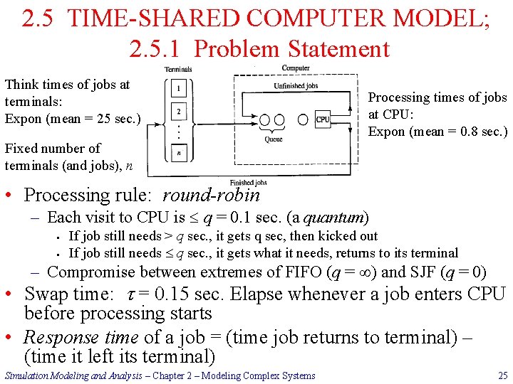
2. 5 TIME-SHARED COMPUTER MODEL; 2. 5. 1 Problem Statement Think times of jobs at terminals: Expon (mean = 25 sec. ) Processing times of jobs at CPU: Expon (mean = 0. 8 sec. ) Fixed number of terminals (and jobs), n • Processing rule: round-robin – Each visit to CPU is q = 0. 1 sec. (a quantum) § § If job still needs > q sec. , it gets q sec, then kicked out If job still needs q sec. , it gets what it needs, returns to its terminal – Compromise between extremes of FIFO (q = ) and SJF (q = 0) • Swap time: = 0. 15 sec. Elapse whenever a job enters CPU before processing starts • Response time of a job = (time job returns to terminal) – (time it left its terminal) Simulation Modeling and Analysis – Chapter 2 – Modeling Complex Systems 25

2. 5. 1 Problem Statement (cont’d. ) • Initially, computer empty and idle, all n jobs in the think state at their terminals • Stopping rule: 1000 response times collected • Output: – Average of the response times – Time-average number of jobs in queue for the CPU – CPU utilization • Question: how many terminals (n) can be loaded on and hold average response time to under 30 sec. ? Simulation Modeling and Analysis – Chapter 2 – Modeling Complex Systems 26

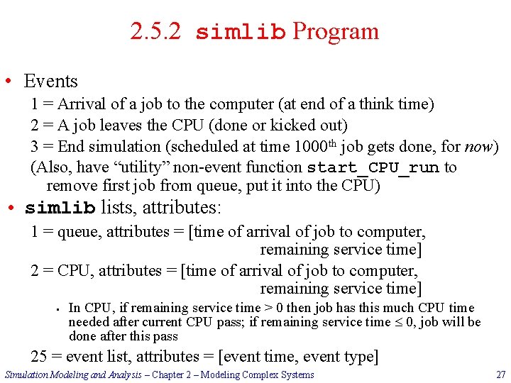
2. 5. 2 simlib Program • Events 1 = Arrival of a job to the computer (at end of a think time) 2 = A job leaves the CPU (done or kicked out) 3 = End simulation (scheduled at time 1000 th job gets done, for now) (Also, have “utility” non-event function start_CPU_run to remove first job from queue, put it into the CPU) • simlib lists, attributes: 1 = queue, attributes = [time of arrival of job to computer, remaining service time] 2 = CPU, attributes = [time of arrival of job to computer, remaining service time] § In CPU, if remaining service time > 0 then job has this much CPU time needed after current CPU pass; if remaining service time 0, job will be done after this pass 25 = event list, attributes = [event time, event type] Simulation Modeling and Analysis – Chapter 2 – Modeling Complex Systems 27

2. 5. 2 simlib Program (cont’d. ); 2. 5. 3 Simulation Output and Discussion • sampst variable: 1 = response times • timest variables: none (use filest or out_filest) • Random-number streams: 1 = think times, 2 = service times • Refer to pp. 133 -141 in the book (Figures 2. 15 -2. 24) and the file tscomp. c – – – – Figure 2. 15 – external definitions (at top of file) Figure 2. 16 – function main Figure 2. 18 – function arrive (flowchart: Figure 2. 17) Figure 2. 20 – function start_cpu_run (flowchart: Figure 2. 19) Figure 2. 22 – function end_cpu_run (flowchart: Figure 2. 21) Figure 2. 23 – function report Figure 2. 24 – output report tscomp. out § Looks like max n is a little under 60 – sure? Simulation Modeling and Analysis – Chapter 2 – Modeling Complex Systems 28

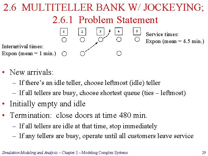
2. 6 MULTITELLER BANK W/ JOCKEYING; 2. 6. 1 Problem Statement Interarrival times: Expon (mean = 1 min. ) Service times: Expon (mean = 4. 5 min. ) • New arrivals: – If there’s an idle teller, choose leftmost (idle) teller – If all tellers are busy, choose shortest queue (ties – leftmost) • Initially empty and idle • Termination: close doors at time 480 min. – If all tellers are idle at that time, stop immediately – If any tellers are busy, operate until all customers leave service Simulation Modeling and Analysis – Chapter 2 – Modeling Complex Systems 29

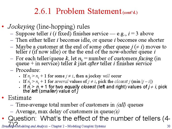
2. 6. 1 Problem Statement (cont’d. ) • Jockeying (line-hopping) rules – Suppose teller i (i fixed) finishes service — e. g. , i = 3 above – Then either teller i becomes idle, or queue i becomes one shorter – Maybe a customer at the end of some other queue j ( i) moves to teller i (if now idle) or the end of the now-shorter queue i – For each teller/queue k, let nk = number of customers facing (in queue + in service) teller k just after teller i finishes service – Procedure: § § § If nj > ni + 1 for some j i, then a jockey will occur If nj > ni + 1 for several values of j i, pick the closest j (min |j – i|) If nj > ni + 1 for two equally closest (left and right) values of j i, pick the left (smaller) value of j • Estimate – Time-average total number of customers in (all) queues – Average, max delay of customers in queue(s) • Question: What’s the effect of the number of tellers (47)? Modeling and Analysis – Chapter 2 – Modeling Complex Systems Simulation 30

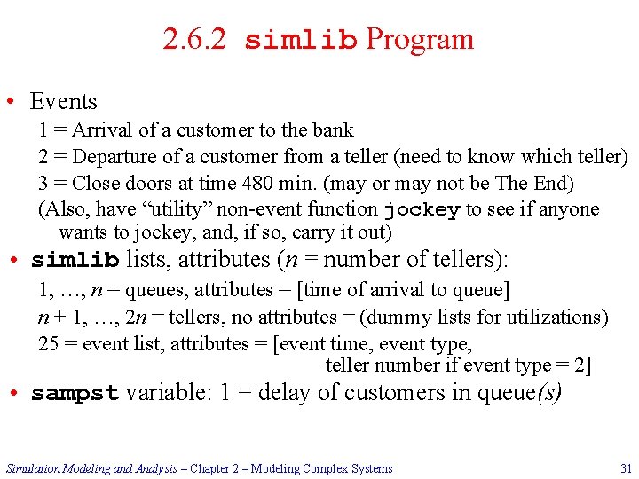
2. 6. 2 simlib Program • Events 1 = Arrival of a customer to the bank 2 = Departure of a customer from a teller (need to know which teller) 3 = Close doors at time 480 min. (may or may not be The End) (Also, have “utility” non-event function jockey to see if anyone wants to jockey, and, if so, carry it out) • simlib lists, attributes (n = number of tellers): 1, …, n = queues, attributes = [time of arrival to queue] n + 1, …, 2 n = tellers, no attributes = (dummy lists for utilizations) 25 = event list, attributes = [event time, event type, teller number if event type = 2] • sampst variable: 1 = delay of customers in queue(s) Simulation Modeling and Analysis – Chapter 2 – Modeling Complex Systems 31

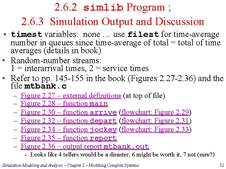
2. 6. 2 simlib Program ; 2. 6. 3 Simulation Output and Discussion • timest variables: none … use filest for time-average number in queues since time-average of total = total of time averages (details in book) • Random-number streams: 1 = interarrival times, 2 = service times • Refer to pp. 145 -155 in the book (Figures 2. 27 -2. 36) and the file mtbank. c – – – – Figure 2. 27 – external definitions (at top of file) Figure 2. 28 – function main Figure 2. 30 – function arrive (flowchart: Figure 2. 29) Figure 2. 32 – function depart (flowchart: Figure 2. 31) Figure 2. 34 – function jockey (flowchart: Figure 2. 33) Figure 2. 35 – function report Figure 2. 36 – output report mtbank. out § Looks like 4 tellers would be a disaster, 6 might be worth it, 7 not (sure? ) Simulation Modeling and Analysis – Chapter 2 – Modeling Complex Systems 32

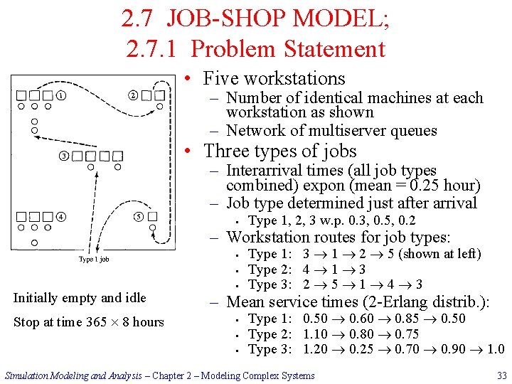
2. 7 JOB-SHOP MODEL; 2. 7. 1 Problem Statement • Five workstations – Number of identical machines at each workstation as shown – Network of multiserver queues • Three types of jobs – Interarrival times (all job types combined) expon (mean = 0. 25 hour) – Job type determined just after arrival § Type 1, 2, 3 w. p. 0. 3, 0. 5, 0. 2 – Workstation routes for job types: § § Initially empty and idle Stop at time 365 8 hours § Type 1: 3 1 2 5 (shown at left) Type 2: 4 1 3 Type 3: 2 5 1 4 3 – Mean service times (2 -Erlang distrib. ): § § § Type 1: 0. 50 0. 60 0. 85 0. 50 Type 2: 1. 10 0. 80 0. 75 Type 3: 1. 20 0. 25 0. 70 0. 90 1. 0 Simulation Modeling and Analysis – Chapter 2 – Modeling Complex Systems 33

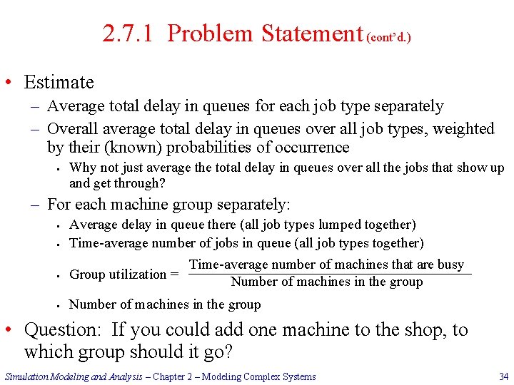
2. 7. 1 Problem Statement (cont’d. ) • Estimate – Average total delay in queues for each job type separately – Overall average total delay in queues over all job types, weighted by their (known) probabilities of occurrence § Why not just average the total delay in queues over all the jobs that show up and get through? – For each machine group separately: § § Average delay in queue there (all job types lumped together) Time-average number of jobs in queue (all job types together) Time-average number of machines that are busy Group utilization = Number of machines in the group • Question: If you could add one machine to the shop, to which group should it go? Simulation Modeling and Analysis – Chapter 2 – Modeling Complex Systems 34

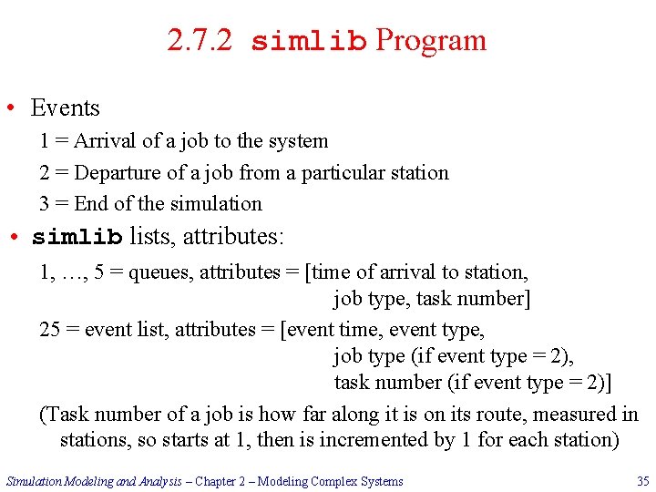
2. 7. 2 simlib Program • Events 1 = Arrival of a job to the system 2 = Departure of a job from a particular station 3 = End of the simulation • simlib lists, attributes: 1, …, 5 = queues, attributes = [time of arrival to station, job type, task number] 25 = event list, attributes = [event time, event type, job type (if event type = 2), task number (if event type = 2)] (Task number of a job is how far along it is on its route, measured in stations, so starts at 1, then is incremented by 1 for each station) Simulation Modeling and Analysis – Chapter 2 – Modeling Complex Systems 35

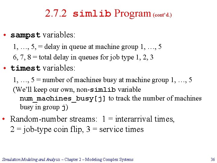
2. 7. 2 simlib Program (cont’d. ) • sampst variables: 1, …, 5, = delay in queue at machine group 1, …, 5 6, 7, 8 = total delay in queues for job type 1, 2, 3 • timest variables: 1, …, 5 = number of machines busy at machine group 1, …, 5 (We’ll keep our own, non-simlib variable num_machines_busy[j] to track the number of machines busy in group j) • Random-number streams: 1 = interarrival times, 2 = job-type coin flip, 3 = service times Simulation Modeling and Analysis – Chapter 2 – Modeling Complex Systems 36

2. 7. 2 simlib Program (cont’d. ); 2. 7. 3 Simulation Output and Discussion • Refer to pp. 160 -169 in the book (Figures 2. 39 -2. 46) and the file jobshop. c – Figure 2. 39 – external definitions (at top of file) – Figure 2. 40 – function main – Figure 2. 42 – function arrive (flowchart: Figure 2. 41) § Note that arrive serves two purposes – new arrival event, “arrival” of an “old” job to its next machine group – Figure 2. 44 – function depart (flowchart: Figure 2. 43) § Note that depart (and this function) is the event of leaving a particular machine group, which may or may not be the end of the road for a job – Figure 2. 45 – function report – Figure 2. 46 – output report mtbank. out § § Looks like congested machine groups are 1, 2, and 4 (sure? ) Reruns with extra machine at each of these in turn – add machine to 4 (? ) Simulation Modeling and Analysis – Chapter 2 – Modeling Complex Systems 37

2. 8 EFFICIENT EVENT-LIST MANIPULATION • Have seen two different ways to store, handle the event list – Sequential by event type – search for smallest entry for next event § Must always look at the whole event list – Ranked in increasing order by event time – insert correctly, take next event from top § Event insertion might not require looking at the whole list • In large simulations with many events, event-list processing can consume much of the total computing time (e. g. , 40%) – Generally worth it to try hard to manage the event list efficiently – Better methods – binary search, storing event list as a tree or heap – Exploit special structure of model to speed up event-list processing § e. g. , if time a record stays on event list is approximately the same for all events, insert a new event via a bottom-to-top search Simulation Modeling and Analysis – Chapter 2 – Modeling Complex Systems 38