Chapter 10 Simulation Modeling 2007 Pearson Education Simulation

Chapter 10: Simulation Modeling © 2007 Pearson Education

Simulation • To simulate is to try to duplicate the characteristics of a real system • We will study mathematical simulation models of real systems to help make business decisions • Simulation is one of the most widely used decision modeling techniques

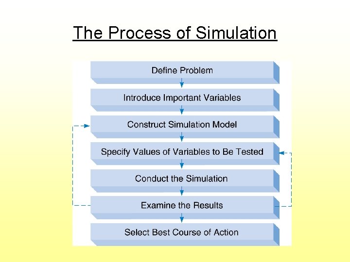
The Process of Simulation

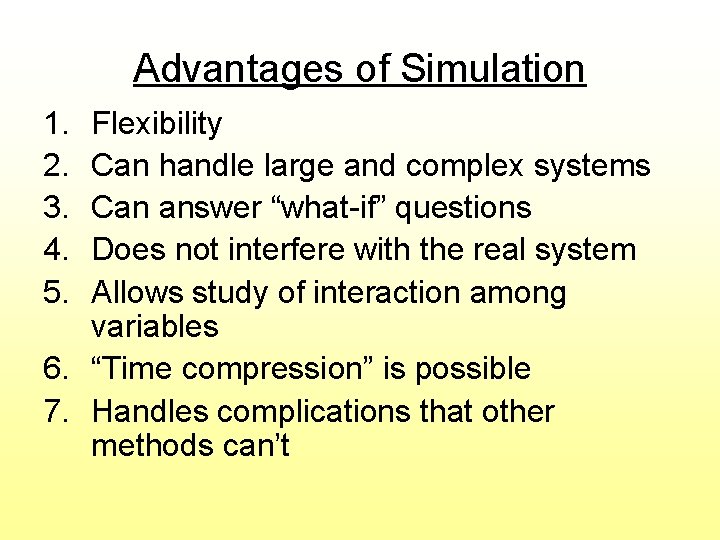
Advantages of Simulation 1. 2. 3. 4. 5. Flexibility Can handle large and complex systems Can answer “what-if” questions Does not interfere with the real system Allows study of interaction among variables 6. “Time compression” is possible 7. Handles complications that other methods can’t

Disadvantages of Simulation 1. Can be expensive and time consuming 2. Does not generate optimal solutions 3. Managers must choose solutions they want to try (“what-if” scenarios) 4. Each model is unique

Monte Carlo Simulation • • Can be used with variables that are probabilistic Steps: 1. Determine the probability distribution for each random variable 2. Use random numbers to generate random values 3. Repeat for some number of replications

Random Variables (RV’s) There are many random variables in real life where there is uncertainty, such as: – Product demand – Lead time for orders – Time between equipment breakdown – Service time – Etc.

Step 1: Determine the Probability Distribution for Each RV • There are many different probability distributions (e. g. general discrete, normal, Poisson, uniform, exponential, binomial, etc. ) • Usually use historical data to determine which distribution “fits” best

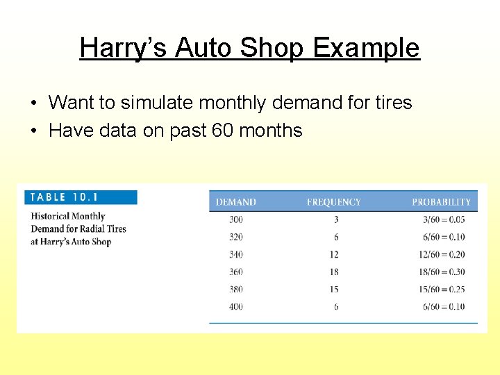
Harry’s Auto Shop Example • Want to simulate monthly demand for tires • Have data on past 60 months

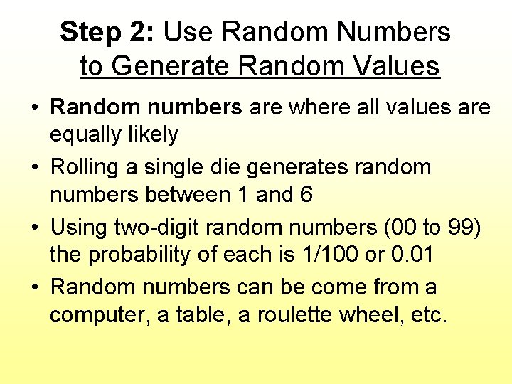
Step 2: Use Random Numbers to Generate Random Values • Random numbers are where all values are equally likely • Rolling a single die generates random numbers between 1 and 6 • Using two-digit random numbers (00 to 99) the probability of each is 1/100 or 0. 01 • Random numbers can be come from a computer, a table, a roulette wheel, etc.

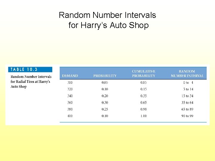
Random Number Intervals for Harry’s Auto Shop

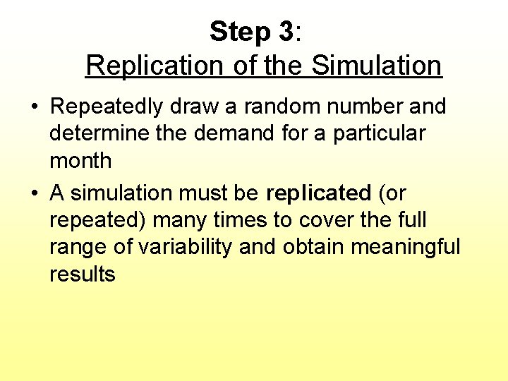
Step 3: Replication of the Simulation • Repeatedly draw a random number and determine the demand for a particular month • A simulation must be replicated (or repeated) many times to cover the full range of variability and obtain meaningful results

Role of Computers in Simulation • The Harry’s example was done “by hand” • Computers are much faster • Software packages have built-in procedures for a variety of probability distributions • Replications are kept track of

Simulation Software Packages • General purpose languages (Visual Basic, C++, Fortran, etc. ) • Special purpose languages and programs (GPSS, Simscript, Microsaint, Build. Sim, etc. ) • Spreadsheet models

Generating Random Values in Excel • To generate random numbers between 0 and 1, use: = RAND() • Using this with various formulas allows generating RV’s from a variety of distributions, including normal, uniform, exponential, and general discrete Go to Excel

Return to Harry’s Auto Shop • Want to compute expected profit • Revenue per tire varies with market conditions – Discrete uniform distribution $60 to $80 • Profit margin per tire also varies – Continuous uniform distribution, 20% to 30% • Fixed operating cost is $2000 per month

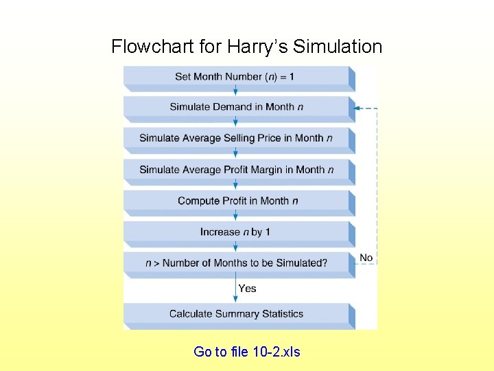
Flowchart for Harry’s Simulation Go to file 10 -2. xls

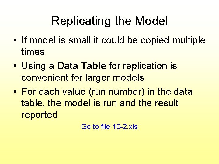
Replicating the Model • If model is small it could be copied multiple times • Using a Data Table for replication is convenient for larger models • For each value (run number) in the data table, the model is run and the result reported Go to file 10 -2. xls

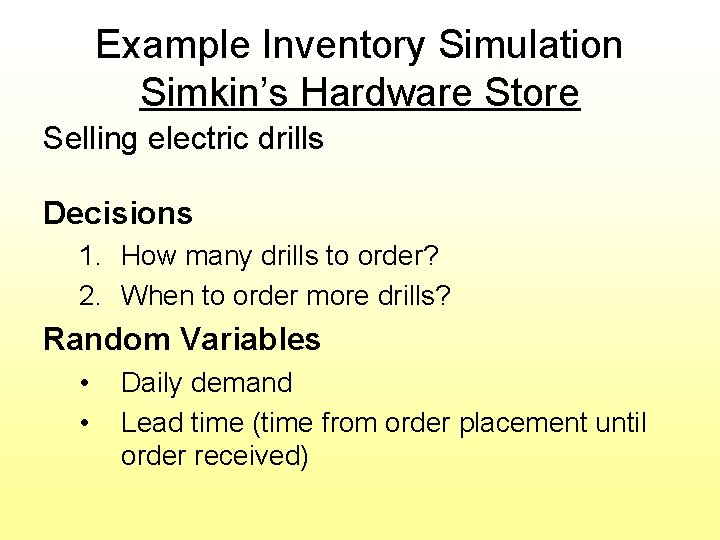
Example Inventory Simulation Simkin’s Hardware Store Selling electric drills Decisions 1. How many drills to order? 2. When to order more drills? Random Variables • • Daily demand Lead time (time from order placement until order received)

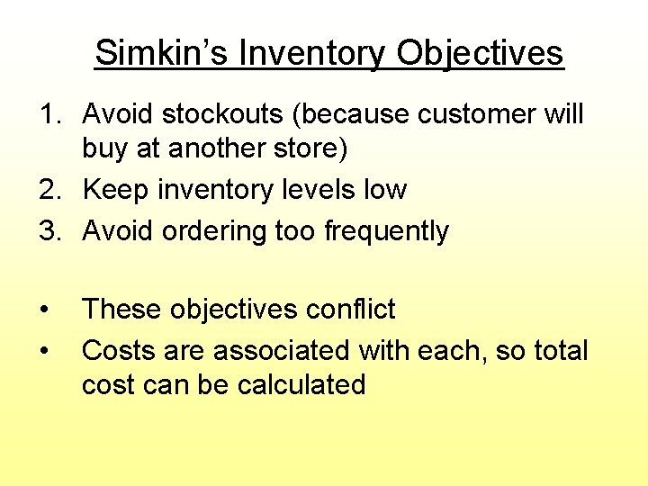
Simkin’s Inventory Objectives 1. Avoid stockouts (because customer will buy at another store) 2. Keep inventory levels low 3. Avoid ordering too frequently • • These objectives conflict Costs are associated with each, so total cost can be calculated

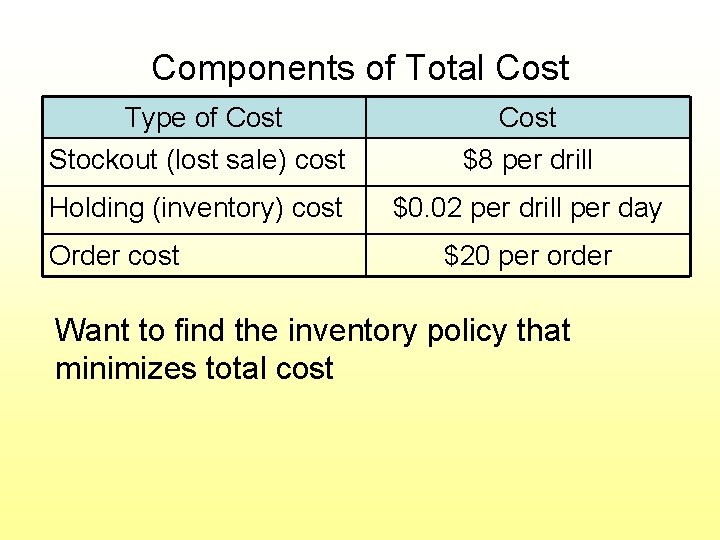
Components of Total Cost Type of Cost Stockout (lost sale) cost Cost $8 per drill Holding (inventory) cost $0. 02 per drill per day Order cost $20 per order Want to find the inventory policy that minimizes total cost

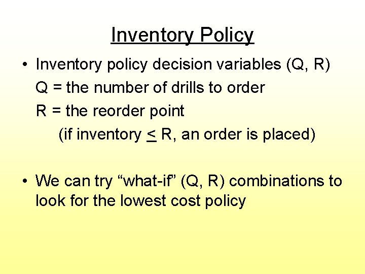
Inventory Policy • Inventory policy decision variables (Q, R) Q = the number of drills to order R = the reorder point (if inventory < R, an order is placed) • We can try “what-if” (Q, R) combinations to look for the lowest cost policy

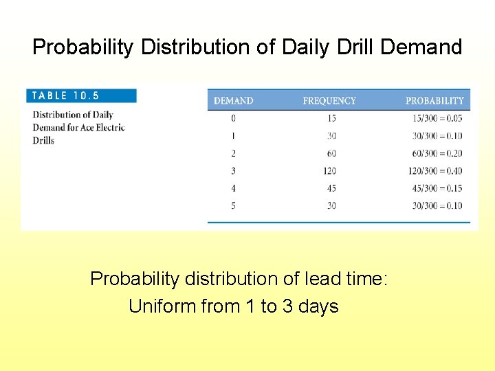
Probability Distribution of Daily Drill Demand Probability distribution of lead time: Uniform from 1 to 3 days

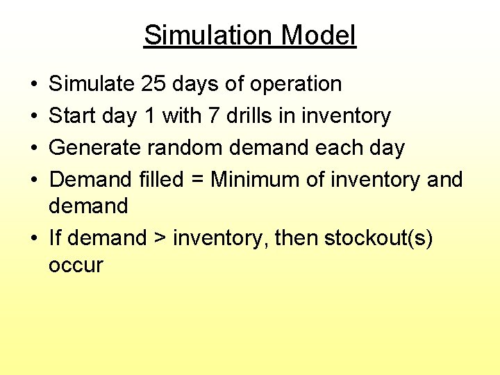
Simulation Model • • Simulate 25 days of operation Start day 1 with 7 drills in inventory Generate random demand each day Demand filled = Minimum of inventory and demand • If demand > inventory, then stockout(s) occur

Simulation Model • Track inventory level – Reduced when drills are sold – Increased when orders arrive • Place an order for Q drills if the day’s ending inventory < R • Each time an order is placed, generate a random value for lead time • Calculate all 3 types of cost and sum for total cost Go to file 10 -3. xls

Replication Using Data Table • Can record all 4 costs (holding, stockout, order, and total cost) for each replication • Each replication represents one month (25 days) of operation • Generate 200 replications Go to file 10 -3. xls

Using Scenario Manager to Include Decisions in Simulation • • Decision variables for Simkin (Q, R) Try Q values 8, 10, 12, and 14 Try R values of 5 and 8 Excel’s Scenario Manager can automatically run all 8 combinations of Q and R Go to file 10 -3. xls

Example Queuing Simulation Denton Savings Bank • • Banks customers arrive randomly and have random service times Customer satisfaction criteria: 1. Average waiting time < 2 minutes 2. Average queue length < 2 customers • Simulate bank operation to determine if criteria are met

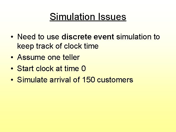
Simulation Issues • Need to use discrete event simulation to keep track of clock time • Assume one teller • Start clock at time 0 • Simulate arrival of 150 customers

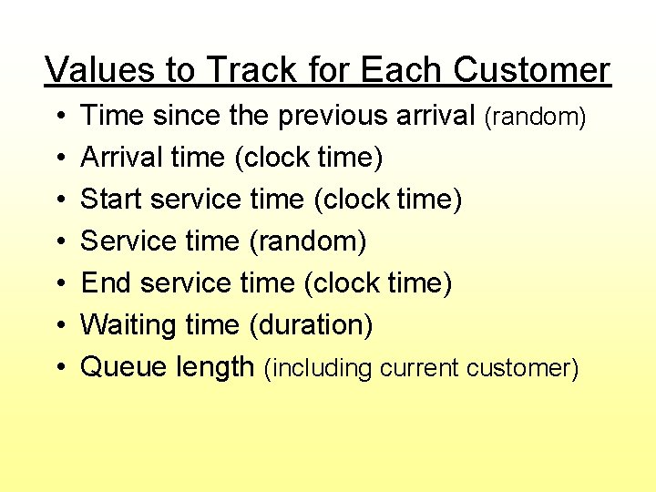
Values to Track for Each Customer • • Time since the previous arrival (random) Arrival time (clock time) Start service time (clock time) Service time (random) End service time (clock time) Waiting time (duration) Queue length (including current customer)

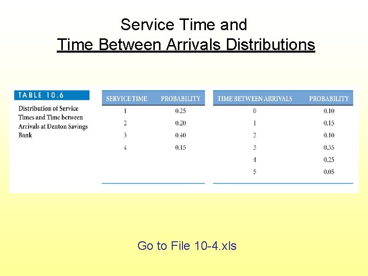
Service Time and Time Between Arrivals Distributions Go to File 10 -4. xls

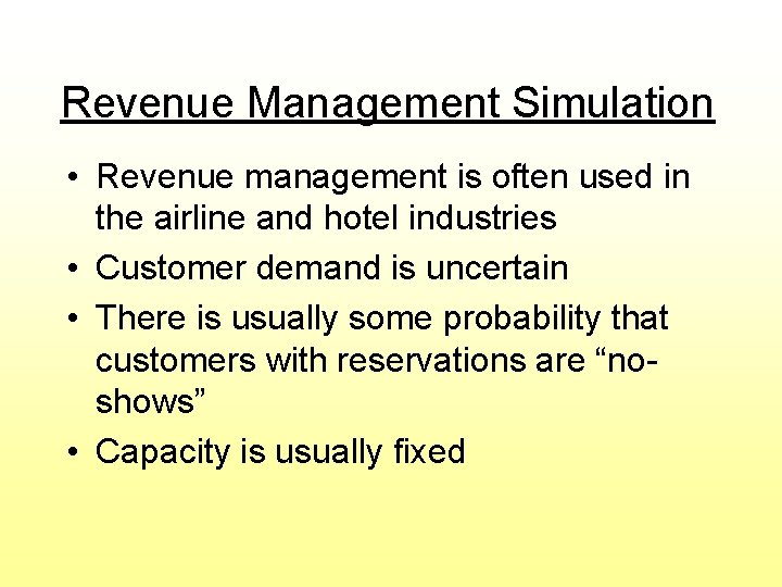
Revenue Management Simulation • Revenue management is often used in the airline and hotel industries • Customer demand is uncertain • There is usually some probability that customers with reservations are “noshows” • Capacity is usually fixed

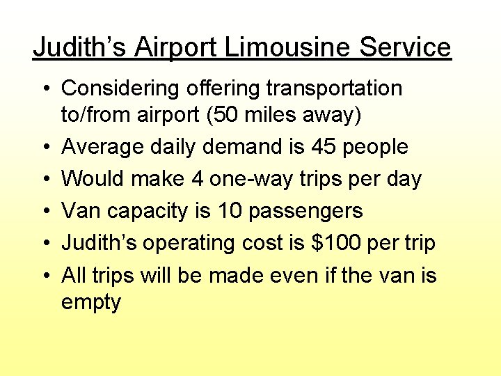
Judith’s Airport Limousine Service • Considering offering transportation to/from airport (50 miles away) • Average daily demand is 45 people • Would make 4 one-way trips per day • Van capacity is 10 passengers • Judith’s operating cost is $100 per trip • All trips will be made even if the van is empty

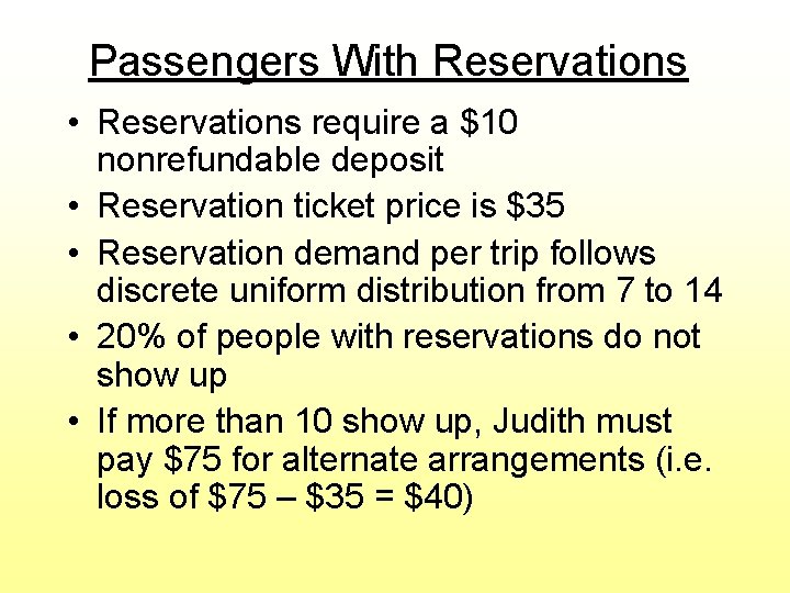
Passengers With Reservations • Reservations require a $10 nonrefundable deposit • Reservation ticket price is $35 • Reservation demand per trip follows discrete uniform distribution from 7 to 14 • 20% of people with reservations do not show up • If more than 10 show up, Judith must pay $75 for alternate arrangements (i. e. loss of $75 – $35 = $40)

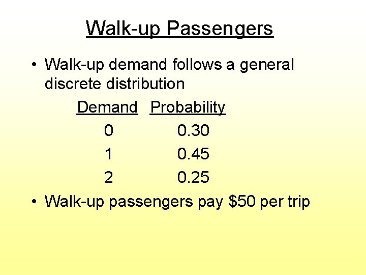
Walk-up Passengers • Walk-up demand follows a general discrete distribution Demand Probability 0 0. 30 1 0. 45 2 0. 25 • Walk-up passengers pay $50 per trip

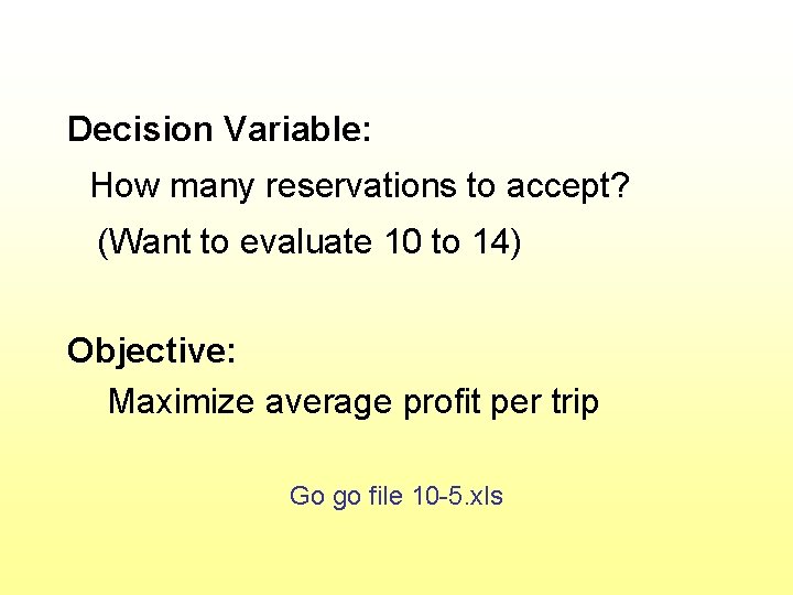
Decision Variable: How many reservations to accept? (Want to evaluate 10 to 14) Objective: Maximize average profit per trip Go go file 10 -5. xls

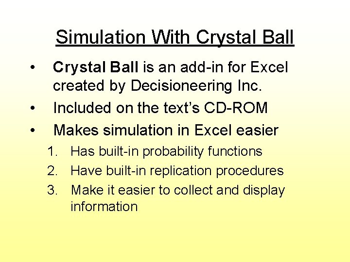
Simulation With Crystal Ball • • • Crystal Ball is an add-in for Excel created by Decisioneering Included on the text’s CD-ROM Makes simulation in Excel easier 1. Has built-in probability functions 2. Have built-in replication procedures 3. Make it easier to collect and display information

Using Crystal Ball • Install from the CD-ROM • Start Crystal Ball • You will be in Excel but an additional menu bar will appear for Crystal Ball

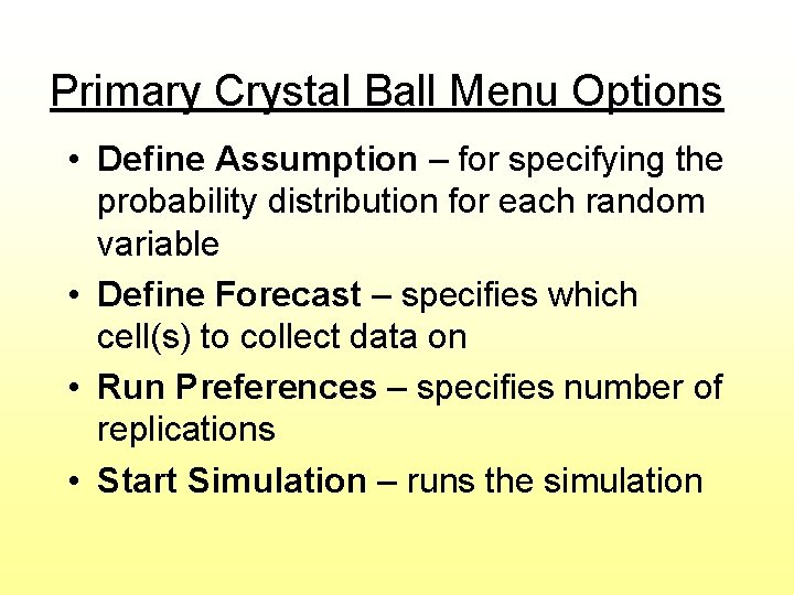
Primary Crystal Ball Menu Options • Define Assumption – for specifying the probability distribution for each random variable • Define Forecast – specifies which cell(s) to collect data on • Run Preferences – specifies number of replications • Start Simulation – runs the simulation

Simkin’s Hardware Store With Crystal Ball • Revisit Simkin’s inventory problem for selling drills • Want to evaluate: – Q (order quantity) values of 8, 10, 12, and 14 – R (reorder point) values of 5 and 8

Simkin’s Hardware Store With Crystal Ball • Use the custom distribution for daily demand • Collect data on (Define Forecast) for: holding cost, stock out cost, order cost, and total cost Go to file 10 -6. xls

Simulation of Revenue Management With Crystal Ball • Revisit Judith’s Limousine service • Use binomial distribution for number of no-show reservations (p=0. 8) • Use the custom distribution for number of walk-ups • Collect data (Define Forecast) for both profit and occupancy rate Go to file 10 -7. xls

Other Types of Simulation Models • Operational Gaming – where there are 2 or more competing players (such as military games or business games) • Systems Simulation – models the dynamics of a large system (more complex than the Monte Carlo methods we have studied)