Ch 3 1 Second Order Linear Homogeneous Equations

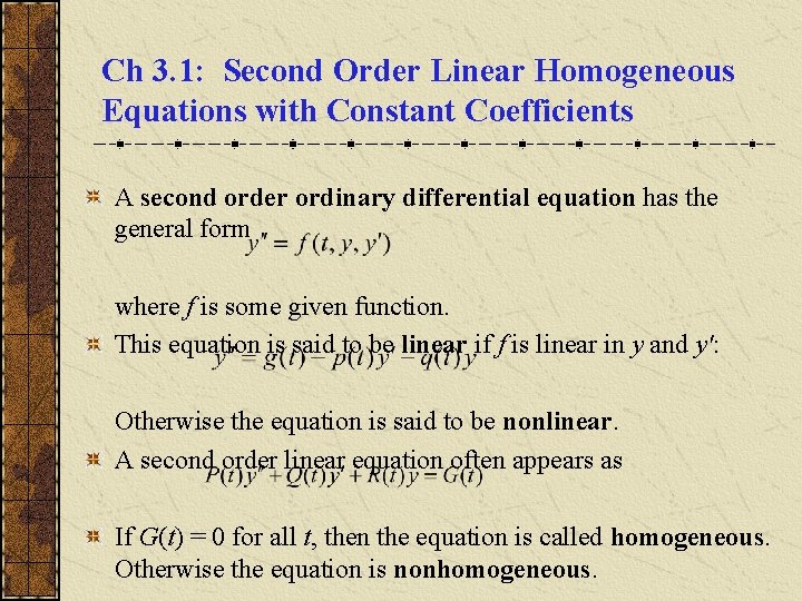
Ch 3. 1: Second Order Linear Homogeneous Equations with Constant Coefficients A second order ordinary differential equation has the general form where f is some given function. This equation is said to be linear if f is linear in y and y': Otherwise the equation is said to be nonlinear. A second order linear equation often appears as If G(t) = 0 for all t, then the equation is called homogeneous. Otherwise the equation is nonhomogeneous.

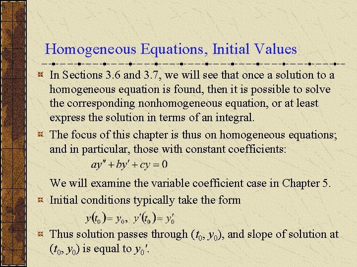
Homogeneous Equations, Initial Values In Sections 3. 6 and 3. 7, we will see that once a solution to a homogeneous equation is found, then it is possible to solve the corresponding nonhomogeneous equation, or at least express the solution in terms of an integral. The focus of this chapter is thus on homogeneous equations; and in particular, those with constant coefficients: We will examine the variable coefficient case in Chapter 5. Initial conditions typically take the form Thus solution passes through (t 0, y 0), and slope of solution at (t 0, y 0) is equal to y 0'.

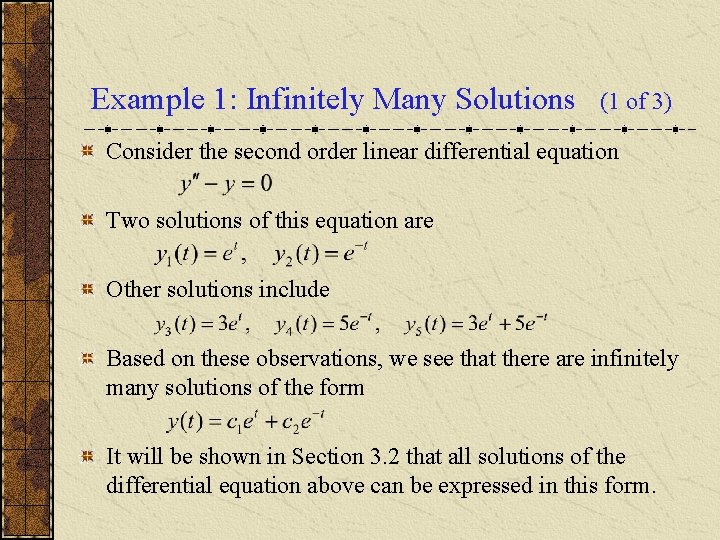
Example 1: Infinitely Many Solutions (1 of 3) Consider the second order linear differential equation Two solutions of this equation are Other solutions include Based on these observations, we see that there are infinitely many solutions of the form It will be shown in Section 3. 2 that all solutions of the differential equation above can be expressed in this form.

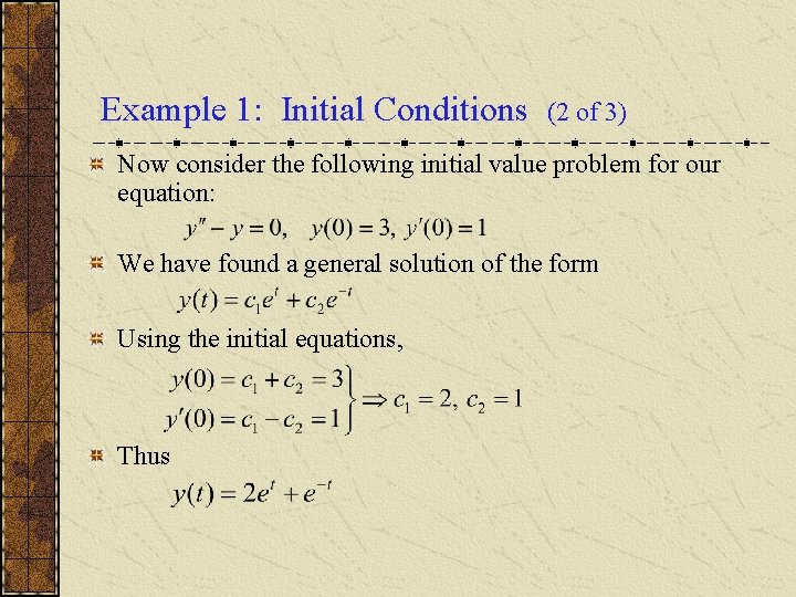
Example 1: Initial Conditions (2 of 3) Now consider the following initial value problem for our equation: We have found a general solution of the form Using the initial equations, Thus

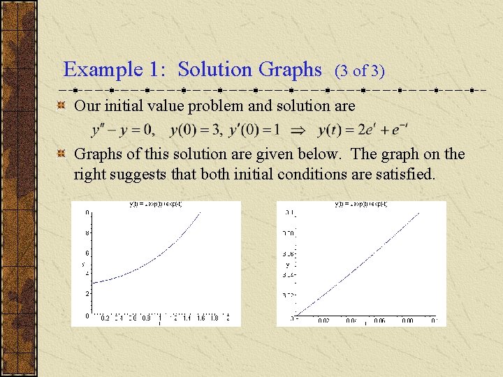
Example 1: Solution Graphs (3 of 3) Our initial value problem and solution are Graphs of this solution are given below. The graph on the right suggests that both initial conditions are satisfied.

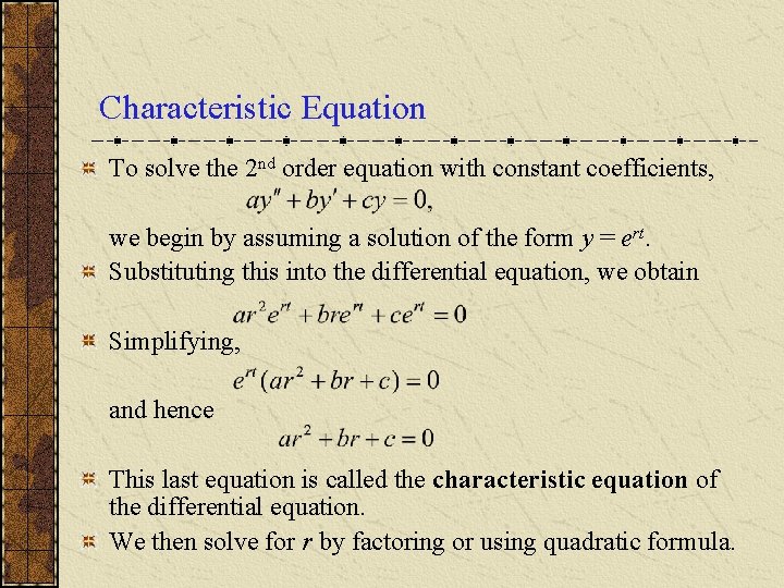
Characteristic Equation To solve the 2 nd order equation with constant coefficients, we begin by assuming a solution of the form y = ert. Substituting this into the differential equation, we obtain Simplifying, and hence This last equation is called the characteristic equation of the differential equation. We then solve for r by factoring or using quadratic formula.

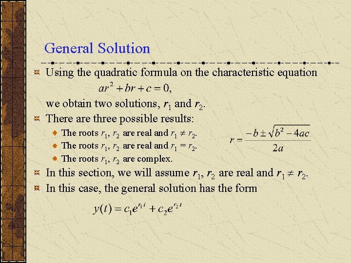
General Solution Using the quadratic formula on the characteristic equation we obtain two solutions, r 1 and r 2. There are three possible results: The roots r 1, r 2 are real and r 1 r 2. The roots r 1, r 2 are real and r 1 = r 2. The roots r 1, r 2 are complex. In this section, we will assume r 1, r 2 are real and r 1 r 2. In this case, the general solution has the form

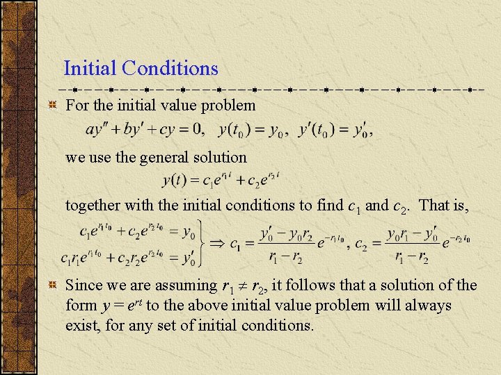
Initial Conditions For the initial value problem we use the general solution together with the initial conditions to find c 1 and c 2. That is, Since we are assuming r 1 r 2, it follows that a solution of the form y = ert to the above initial value problem will always exist, for any set of initial conditions.

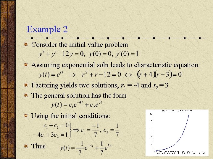
Example 2 Consider the initial value problem Assuming exponential soln leads to characteristic equation: Factoring yields two solutions, r 1 = -4 and r 2 = 3 The general solution has the form Using the initial conditions: Thus

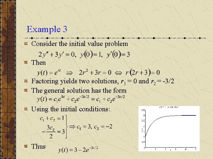
Example 3 Consider the initial value problem Then Factoring yields two solutions, r 1 = 0 and r 2 = -3/2 The general solution has the form Using the initial conditions: Thus

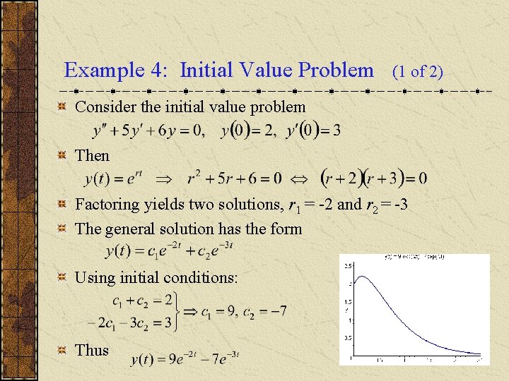
Example 4: Initial Value Problem (1 of 2) Consider the initial value problem Then Factoring yields two solutions, r 1 = -2 and r 2 = -3 The general solution has the form Using initial conditions: Thus

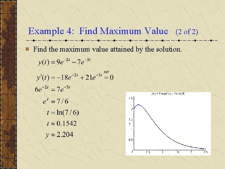
Example 4: Find Maximum Value (2 of 2) Find the maximum value attained by the solution.