CERI7104CIVL8126 Data Analysis in Geophysics Continue Introduction to

CERI-7104/CIVL-8126 Data Analysis in Geophysics Continue Introduction to Matlab Programming. Lab – 4 b, 09/05/19

More on vectorization. MATLAB is a vectorized high level language Requires change in programming style (if one already knows a non-vectorized programming language such as Fortran, C, Pascal, Basic, etc. ) Vectorized languages allow operations over arrays using simple syntax, essentially the same syntax one would use to operate over scalars. (looks like math again. )

What is vectorization? (with respect to matlab) Vectorization is the process of writing code for MATLAB that uses matrix operations or other fast built-in functions instead of using explicit loops. The benefits of doing this are usually sizeable. The reason for this is that MATLAB is an interpreted language. Function calls have very high overhead, and indexing operations (inherent in a loop operation) are not particularly fast.

Loop versus vectorized version of same code. New commands “tic” and “toc” - time the execution of the code between them. >> a=rand(1000); >> tic; b=a*a; toc Elapsed time is 0. 229464 seconds. >> tic; for k=1: 1000, for l=1: 1000, c(k, l)=0; for m=1: 1000, c(k, l)=c(k, l)+a(k, m)*a(m, l); end, toc Elapsed time is 22. 369451 seconds. >> whos Name Size Bytes Class Attributes a 1000 x 1000 8000000 double b 1000 x 1000 8000000 double c 1000 x 1000 8000000 double k 1 x 1 8 double l 1 x 1 8 double m 1 x 1 8 double >> max(b-c)) ans = 9. 6634 e-13 Factor 100 difference in time for multiplication of 103 x 103 matrix!

Vectorization of synthetic seismogram example from Stein and Wysession Intro to Seismology and Earth Structure. Section on scientific programming

Start by just "translating" the Fortran code into Matlab. So far we probably don't fully understand the math, but we have a formula and so we can calculate u(x, t).

u(cnt)=0; %synthetic seismogram for homogeneous string, u(t) end %calculated by normal mode summation for k=1: nstep %string length t(k)=dt*(k-1); alngth=1; end %velocity m/sec %outer loop over modes c=1. 0; for n=1: nmode %number modes anpial=n*pi/alngth; nmode=200; %space terms - src & rcvr %source position sxs=sin(anpial*xsrc); xsrc=0. 2; sxr=sin(anpial*xrcvr); %receiver position %mode freq xrcvr=0. 7; wn=n*pi*c/alngth; %seismogram time duration %time indep terms tdurat=1. 25; dmp=(tau*wn)^2; %number time steps scale=exp(-dmp/4); nstep=50; space=sxs*sxr*scale; %time step %inner loop oner time steps dt=tdurat/nstep; for k=1: nstep %source shape term % t=dt*(k-1); tau=0. 02; % cwt=cos(wn*t); fprintf('%sn', 'synthetic seismogram for string') cwt=cos(wn*t(k)); fprintf('%s %0. 5 gn', 'number modes', nmode) fprintf('%s %0. 5 gn', 'length and velocity', alngth, %compute disp u(k)=u(k)+cwt*space; c) end fprintf('%s %0. 5 gn', 'posn src and end rcvr', xsrc, xrcvr) plot(t, u) fprintf('%s %0. 5 gn', 'durn, time steps, del t', tdurat, nstep, dt) fprintf('%s %0. 5 gn', 'source shape', tau) %initialize displacement for cnt=1: nstep Doing translation for homework Slightly cleaned up version of Fortran program in Stein and Wysession “translated” to Matlab. (took calculation of time out of inner loop – is recalculated each time through, waste of time, calculate as vector once at beginning)

Synthetic seismogram produced by Matlab code translated from Fortran.

Variables >> whos Name Size alngth 1 x 1 anpial 1 x 1 cnt 1 x 1 cwt 1 x 1 dmp 1 x 1 dt 1 x 1 k 1 x 1 nmode 1 x 1 nstep 1 x 1 scale 1 x 1 space 1 x 1 sxr 1 x 1 sxs 1 x 1 tau 1 x 1 tdurat 1 x 1 u 1 x 50 wn 1 x 1 xrcvr 1 x 1 xsrc 1 x 1 Bytes Class 8 double 8 double 8 double 8 double 8 double 400 double 8 double Attributes

Let's return to the original problem and try to understand what is going on. We will use this to understanding to further vectorize (speed up) the code.

This is just the Fourier domain representation for waves on a string with fixed ends Weight - no dependence on x or t, only wn. Standing wave made from 2 opposite direction traveling waves. Amplitude varies with time, but does not "move" Going left right Going

Normal Mode (and combination of traveling waves to make standing wave) formulation for displacement of a string This is a sinusoidal wave that is fixed in space, cos(kx), whose amplitude is modulated harmonically in time, cos (ωt)

Do over a range of frequencies. Delta functions going right on top and left in middle and combined (bottom). u(x, t)=Acos (kx+ωt)+Acos(kx−ωt) u(k, ω)=Acos (kx+ωt)+Acos(kx−ωt) u(x, t)=u(k, ω)=2 Acos(ωt)cos(kx)

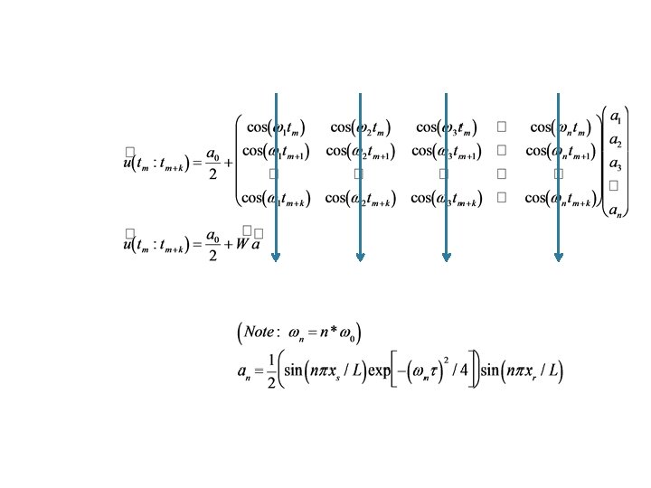
Look at the basic element of Fourier series, weighted sum of sin and cos functions (look at cos only to see how works). Dot product or matrix multiply: ac=(c'a')' matrix multiply, at multiple times to make full seismogram

Look at the basic Fourier series At constant time, weighted sum of cosines at different frequencies at that time constant frequency cosine as function of time (basis functions) This is multiplication of a matrix (with cosines as functions of frequency – across - and time down) times a vector containing the Fourier series weights.

We have just vectorized the equations for the Fourier series!

Even though this is a major improvement over doing this with for loops, and is clear conceptually, it is still not "computable" as it takes O(N 2) operations (and therefore time) to do it. This is OK for small N, but quickly gets out of hand. Fourier analysis is typically done using the Fast Fourier transform (FFT) algorithm – which has O(N log 2 N) operations and is significantly faster for large N.

Fourier decomposition. “Basis” functions are the sine and cosine functions. Notice that first sine term is all zeros (so don’t really need it) and last sine term (not shown) is same as last cosine term, just shifted one – so will only need one of these). Figure from Smith

Fourier transform (actually Fourier series) The Fast Fourier Transform (FFT) depends on noticing that there is a lot of repetition in the calculations – each higher frequency basis function can be made by selecting points from the w 0 function. The weight value is multiplied by the same basis function value an increasing number of times as w increases. Figure from Smith

FFT The FFT uses regularities of the calculation to calculate the basis functions and then basically does each unique multiplication only once, stores it, and then does the bookeeping to add them all up correctly. The points in the trace at the top are made from vertical sums of the weighted points at the same time in the cos and sin traces in the bottom. Figure from Smith

FFT The FFT uses the following symmetry properties Symmetry Periodicity FFT needs number points = power of 2. Figure from Smith

% number of time samples M % points % source/receiver position: % xs/xr (meters) % speed c (meters/sec) % length L (meters) % number of modes N % source pulse duration Tau % (sec) % length of seismogram T (sec) M=50; xs=0. 25; xr = 0. 7; c=1; L=1; N=200; Tau=0. 02; T=1. 25; Same program in Matlab after vectorization (is mostly comments!) %time vector, 1 row by M start, step, stop %will need lots, calc once dt=T/M; t=0: dt: T-dt; %columns:

We need to make the matrix and the vector Making the matrix. What size does it have to be? What does each row and column represent?

There are N=200 columns for the M frequencies There are N=50 rows for the N samples in the seismogram time series. How do we make the elements (k, l) of the matrix? Use fact that values needed are proportional to k and l.

Make appropriate vectors for time and frequency. How big is each? How combine them to make the matrix as a function of k and l?

Multiply elements of the matrix by dt and Take cosine of matrix. .

Now calculate the weights. Note the weights depend on n, and , but not t. All t dependence is in the matrix elements.

So now have matrix with the trigonometric basis functions and a vector of the weights. Just multiply them! (careful with sizes)

This is not the way it is typically done (although some people still do it the "Fortran" way) as it is still O(N 2). The Matlab matrix multiplication method is faster than the Matlab loop method. (a good Fortran compiler will beat the pants off either implementation in Matalb). We did it this way for educational purposes. Typically, it is done using the FFT (Fast Fourier Transform) algorithm which avoids duplication of effort in the multiplications and results in O(N log 2 N) multiplications.

For a time series 216=65, 536 (FFT needs number of points = power of two, this is pretty typical number of points in seismogram, about 10 minutes at 100 Hz sampling) We need O(16 * 216)=1, 048, 576 Vs (216)2= 4, 294, 967, 296 Multiplications (slow) (ratio 2. 44140625 e-4 -> 4096 times faster!!)

Two lessons Vecotorizing Matlab (turn loops into matrix operations) makes Matlab go lots faster. Should do it. Vectorizing in general - is not algorithmic - is case specific can give gigantic speed improvements (much more than Matlab style vectorizing) and even make something that is non-computable, computable. But is lots of work - an art!

Get same figure as before.