CERI7104CIVL8126 Data Analysis in Geophysics Intro Seismic Analysis

CERI-7104/CIVL-8126 Data Analysis in Geophysics Intro “Seismic Analysis Code” - SAC Lab – 20, 11/01/19

First Sharing files between host OS (windows 10 for example) and your virtual machine (UBUNTU in Virtual. Box for example) Google “share folder virtual box and windows” Use a shared folder Use Windows for getting files from network, then access them from the shared folder (both “machines”/”systems” see it and can read/write to it)

SAC (Seismic Analysis Code) General purpose interactive program designed for the study of sequential signals, especially seismic timeseries data (seismograms). Emphasis has been placed on analysis tools used by research seismologists in the detailed study of seismic events.

SAC (Seismic Analysis Code) Analysis capabilities include: - General arithmetic operations -Fourier transforms - integration/differentiation - spectral estimation/processing techniques - IIR and FIR filtering -Signal stacking - Decimation and Interpolation, - Correlation, - seismic phase (time and amplitude) picking - Instrument correction - Particle motion rotation - Trace envelopes - Linear regressions - Frequency-wavenumber analysis - various types of plotting.

SAC It is a command-driven, as opposed to a menu or GUI driven, program. It took advantage of several features of the PRIMEOS (the OS from the computer company PRIME), such as its command line processor that passes commands that are not part of the program to the OS. (This means, that if one is running SAC and you need to get a directory listing, you just enter the “ls” command. Since this is not a SAC command, the command line processor will pass the command to the OS and you will get a directory listing. You don’t have to leave SAC, do the “ls”, write down/remember the file name, and restart SAC. This was very important in the pre –GUI days. )

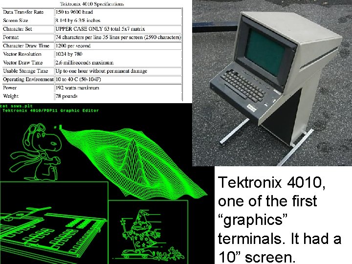
SAC Although it can run in batch mode, it was principally designed to be interactive and have interactive graphics. It was designed to use the “state-of-the-art” Tektronix 401 X “storage tube” line of graphics terminals.

Tektronix 4010, one of the first “graphics” terminals. It had a 10” screen.

SAC After the demise of PRIME in the early 90’s, SAC was beaten into submission to run under the UNIX operating system, specifically, SOLARIS, the SUN (which has followed PRIME into oblivion) OS. (as with UNIX, SAC dragged along many of the idiosyncrasies of its birth associated with the PRIMEOS and the hardware limitations of the time – such as the TEK 401 X. The UNIX implementation was the simplest “make it run” under UNIX effort – amounted to writing a graphics translator from tektronix graphics commands to the current ones – no rethinking, etc. due to new hardware and capabilities – just translate line by line. ) It now runs on most UNIX/LINUX systems and has become one of the standard data manipulation tools in seismology.

SAC data SAC’s data format, especially for binary data, is one of the principle data formats still used in storing, transferring, and manipulating (earthquake) seismological time series data.

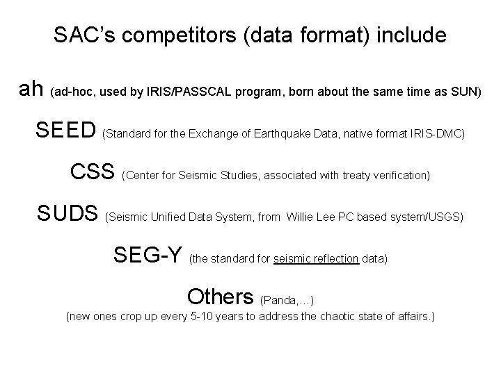
SAC’s competitors (data format) include ah (ad-hoc, used by IRIS/PASSCAL program, born about the same time as SUN) SEED (Standard for the Exchange of Earthquake Data, native format IRIS-DMC) CSS (Center for Seismic Studies, associated with treaty verification) SUDS (Seismic Unified Data System, from Willie Lee PC based system/USGS) SEG-Y (the standard for seismic reflection data) Others (Panda, …) (new ones crop up every 5 -10 years to address the chaotic state of affairs. )

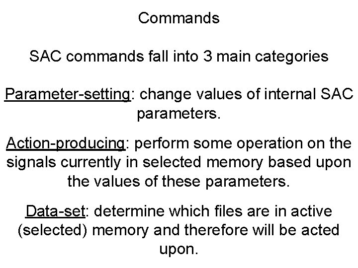
Commands SAC commands fall into 3 main categories Parameter-setting: change values of internal SAC parameters. Action-producing: perform some operation on the signals currently in selected memory based upon the values of these parameters. Data-set: determine which files are in active (selected) memory and therefore will be acted upon.

Commands help calls up a list of all commands. help command shows the manual page for the command.

Data File Command Module This module is used to read, write, and access SAC data files. read (can be shortened to “r”): reads data files from disk into memory sac> r *. SAC Uses standard UNIX wildcards: reads all files whose filenames end in “. SAC”

Data File Command Module write ( “w”): writes the data currently in memory to disk You can write the data into a range of file formats and file names or simply overwrite the current set of files. (so be careful, you’ve been warned)

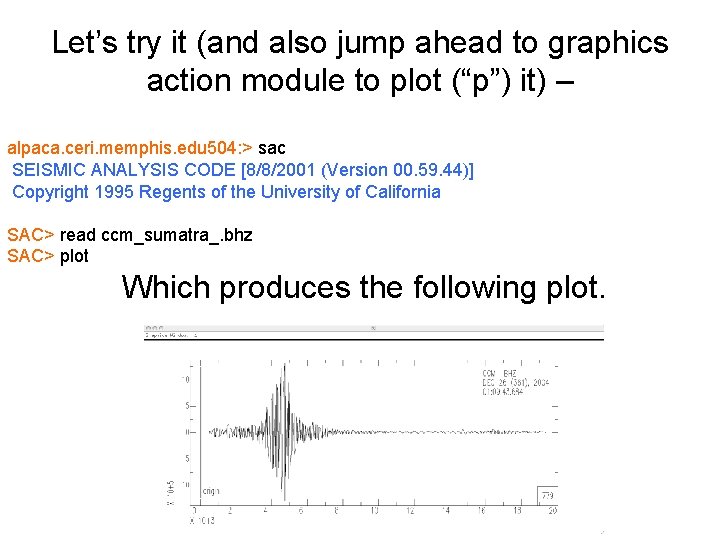
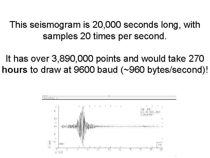
Let’s try it (and also jump ahead to graphics action module to plot (“p”) it) – alpaca. ceri. memphis. edu 504: > sac SEISMIC ANALYSIS CODE [8/8/2001 (Version 00. 59. 44)] Copyright 1995 Regents of the University of California SAC> read ccm_sumatra_. bhz SAC> plot Which produces the following plot.

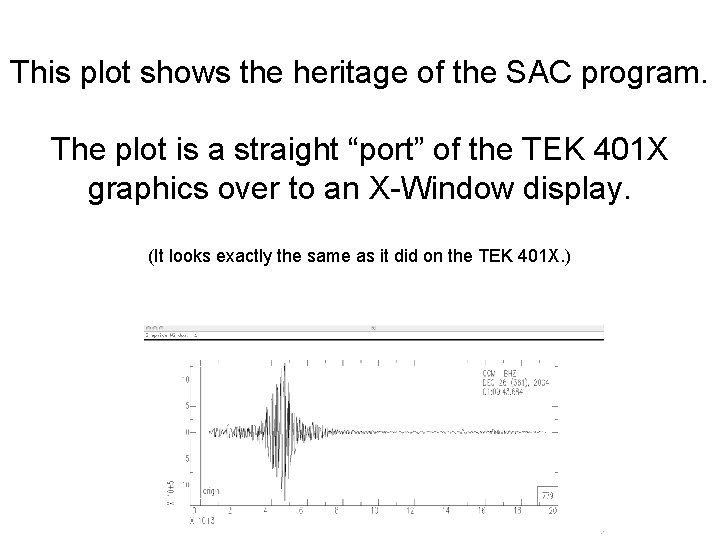
This plot shows the heritage of the SAC program. The plot is a straight “port” of the TEK 401 X graphics over to an X-Window display. (It looks exactly the same as it did on the TEK 401 X. )

This seismogram is 20, 000 seconds long, with samples 20 times per second. It has over 3, 890, 000 points and would take 270 hours to draw at 9600 baud (~960 bytes/second)!

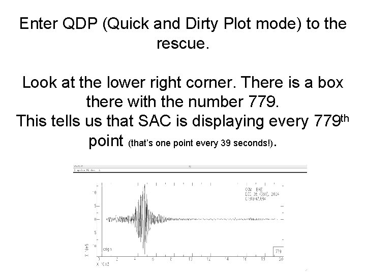
Enter QDP (Quick and Dirty Plot mode) to the rescue. Look at the lower right corner. There is a box there with the number 779. This tells us that SAC is displaying every 779 th point (that’s one point every 39 seconds!).

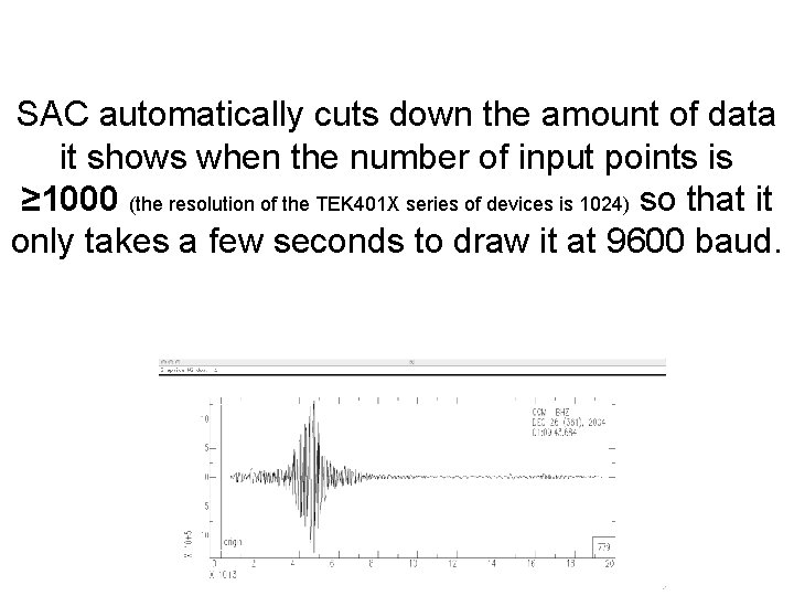
SAC automatically cuts down the amount of data it shows when the number of input points is ≥ 1000 (the resolution of the TEK 401 X series of devices is 1024) so that it only takes a few seconds to draw it at 9600 baud.

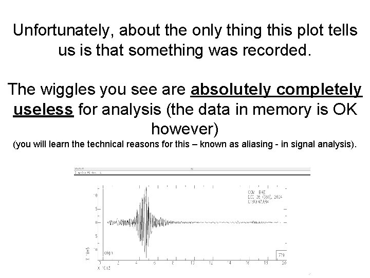
Unfortunately, about the only thing this plot tells us is that something was recorded. The wiggles you see are absolutely completely useless for analysis (the data in memory is OK however) (you will learn the technical reasons for this – known as aliasing - in signal analysis).

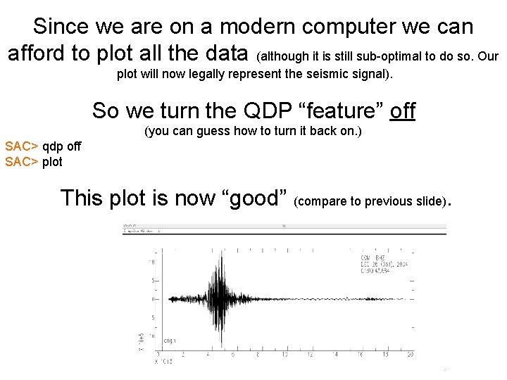
Since we are on a modern computer we can afford to plot all the data (although it is still sub-optimal to do so. Our plot will now legally represent the seismic signal). So we turn the QDP “feature” off (you can guess how to turn it back on. ) SAC> qdp off SAC> plot This plot is now “good” (compare to previous slide).

qdp is the correct idea (don’t waste time displaying stuff that you can’t see due to screen resolution), but it is very badly implemented. qdp should have taken the max and min of each of the sections of N points (instead of each Nth point) and plotted a vertical line between them at each time (it would have taken twice as long to display, but the qdp display was relatively quick). The display would be identical to the full display on the last slide (and look like a paper record). (this would have cost some computer time to calculate what to display, but that is minimal compared to the data transfer time to the TEK 401 X. As it is now it takes the decimation factor longer to calculate what gets drawn on the screen – you don't notice it, but the drawing is instantaneous).

So far we have some files in memory. If we simply read in another file(s) – the new data will clobber what we have. If we need to read in more data (say we have processed the data we’ve read in and now want a spectral ratio of the processed data with the original data) we have to use the “more” option to read in additional data (to not clobber what is there). read more filename

In general SAC does commands to all the files in memory. If the command is starting from scratch (like a read) it clobbers what is already there. Some commands require certain pairs of files (N and E for example for rotating seismograms).

We have now seen 4 SAC commands (but only used 3). read filename write still to be determined plot qdp on or off

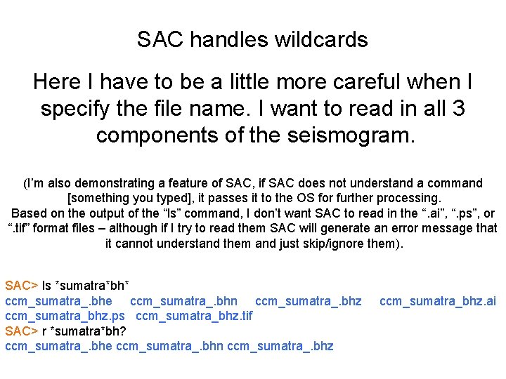
SAC handles wildcards Here I have to be a little more careful when I specify the file name. I want to read in all 3 components of the seismogram. (I’m also demonstrating a feature of SAC, if SAC does not understand a command [something you typed], it passes it to the OS for further processing. Based on the output of the “ls” command, I don’t want SAC to read in the “. ai”, “. ps”, or “. tif” format files – although if I try to read them SAC will generate an error message that it cannot understand them and just skip/ignore them). SAC> ls *sumatra*bh* ccm_sumatra_. bhe ccm_sumatra_. bhn ccm_sumatra_. bhz ccm_sumatra_bhz. ps ccm_sumatra_bhz. tif SAC> r *sumatra*bh? ccm_sumatra_. bhe ccm_sumatra_. bhn ccm_sumatra_. bhz ccm_sumatra_bhz. ai

Fortunately (in the newer versions of UNIX-SAC) the OS handles the command entry and you can still move around through the command line or “history” with the cursor keys and use regular expressions to build names (wildcards, etc. ).

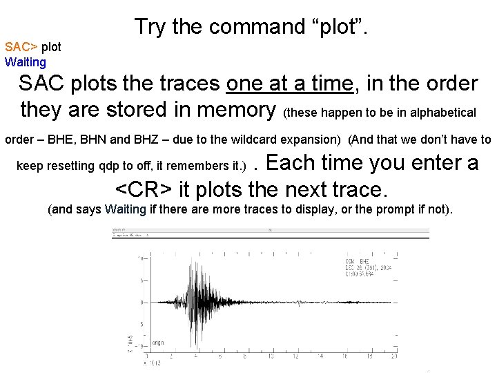
Try the command “plot”. SAC> plot Waiting SAC plots the traces one at a time, in the order they are stored in memory (these happen to be in alphabetical order – BHE, BHN and BHZ – due to the wildcard expansion) (And that we don’t have to . Each time you enter a <CR> it plots the next trace. keep resetting qdp to off, it remembers it. ) (and says Waiting if there are more traces to display, or the prompt if not).

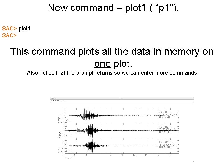
New command – plot 1 ( “p 1”). SAC> plot 1 SAC> This command plots all the data in memory on one plot. Also notice that the prompt returns so we can enter more commands.

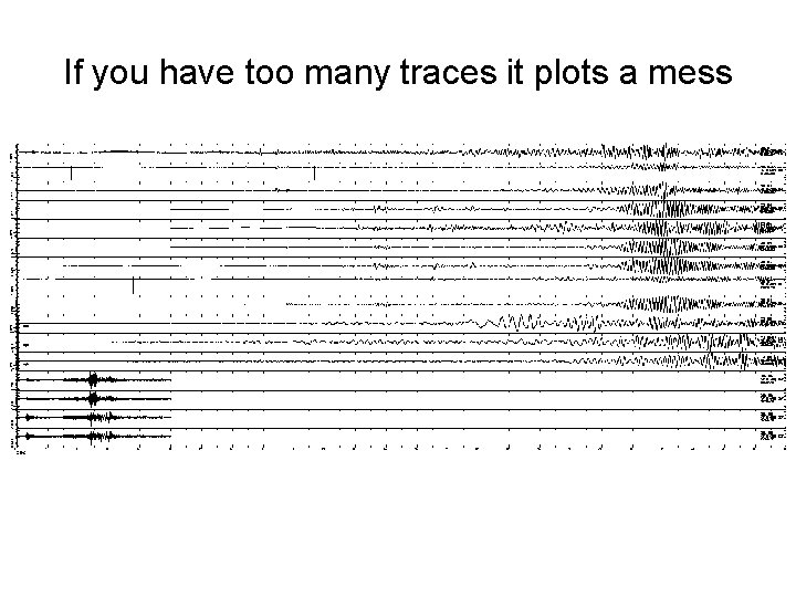
If you have too many traces it plots a mess

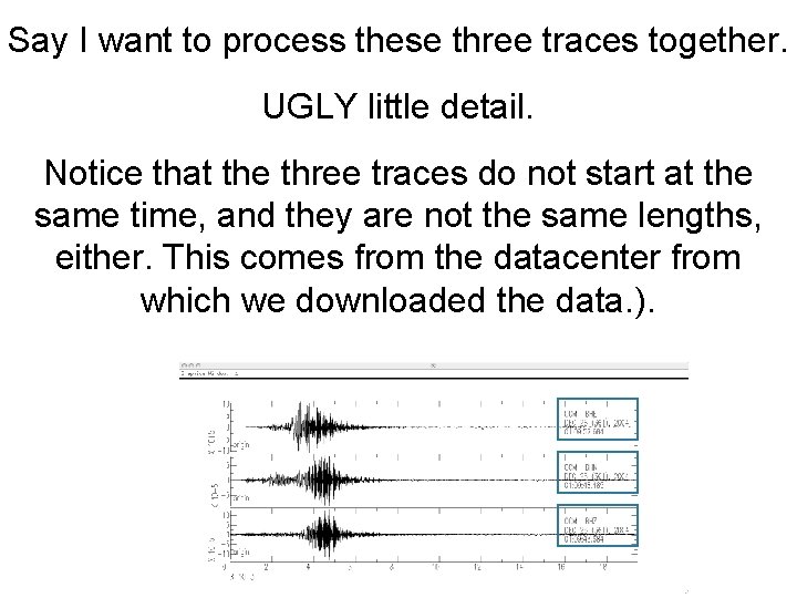
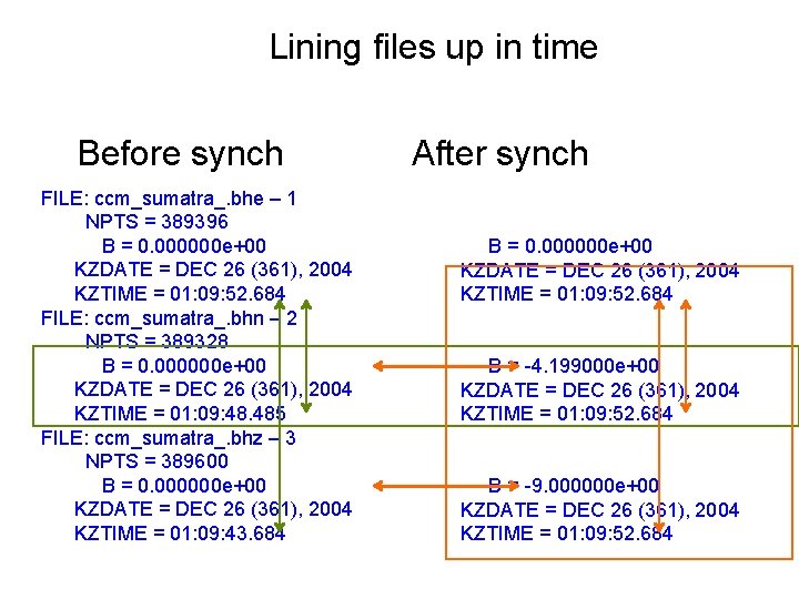
Say I want to process these three traces together. UGLY little detail. Notice that the three traces do not start at the same time, and they are not the same lengths, either. This comes from the datacenter from which we downloaded the data. ).

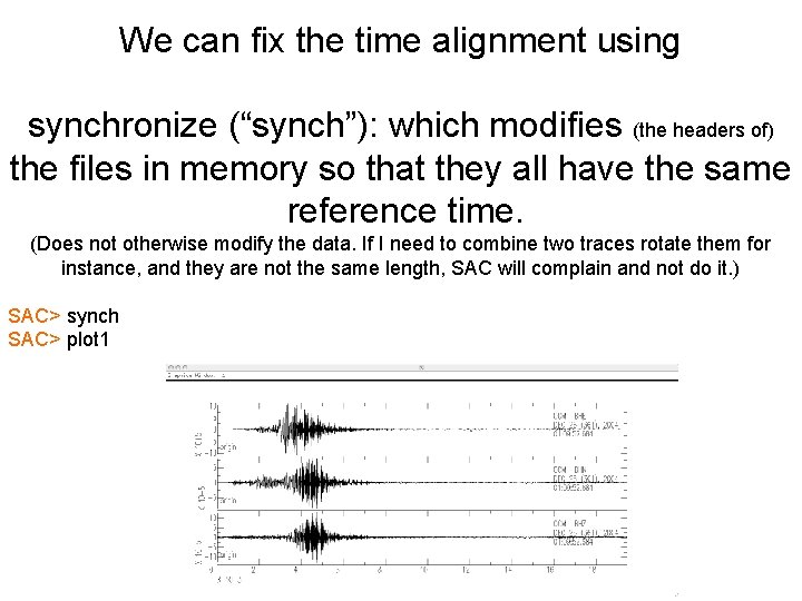
We can fix the time alignment using synchronize (“synch”): which modifies (the headers of) the files in memory so that they all have the same reference time. (Does not otherwise modify the data. If I need to combine two traces rotate them for instance, and they are not the same length, SAC will complain and not do it. ) SAC> synch SAC> plot 1

How do we find out what do we have in memory? What metadata is available about the seismic data? (metadata is data about data – examples are the name of the seismic station and component, the sampling rate, etc. This information is stored in the SAC header. ) listhdr (lh): lists the headers of the files in memory.

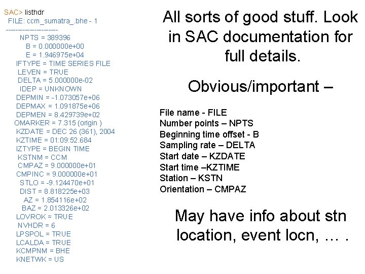
SAC> listhdr FILE: ccm_sumatra_. bhe - 1 -----------NPTS = 389396 B = 0. 000000 e+00 E = 1. 946975 e+04 IFTYPE = TIME SERIES FILE LEVEN = TRUE DELTA = 5. 000000 e-02 IDEP = UNKNOWN DEPMIN = -1. 073057 e+06 DEPMAX = 1. 091875 e+06 DEPMEN = 8. 429739 e+02 OMARKER = 7. 315 (origin ) KZDATE = DEC 26 (361), 2004 KZTIME = 01: 09: 52. 684 IZTYPE = BEGIN TIME KSTNM = CCM CMPAZ = 9. 000000 e+01 CMPINC = 9. 000000 e+01 STLO = -9. 124470 e+01 DIST = 8. 818225 e+03 AZ = 1. 854116 e+02 BAZ = 2. 013326 e+02 LOVROK = TRUE NVHDR = 6 LPSPOL = TRUE LCALDA = TRUE KCMPNM = BHE KNETWK = US All sorts of good stuff. Look in SAC documentation for full details. Obvious/important – File name - FILE Number points – NPTS Beginning time offset - B Sampling rate – DELTA Start date – KZDATE Start time –KZTIME Station – KSTN Orientation – CMPAZ May have info about stn location, event locn, ….

Says Waiting when page is full (may not be complete header listing). <CR> to continue till run out of stuff to display. (there is no way to “break” out of the commands (e. g. : plot, listhdr, …) that do something for each file. You have to <CR> till it finishes, or ^C out and start over. )

Commands to see/change header values listhdr (lh): list the header contents. readhdr (rh) and writehdr (wh): read and write headers without the data. chnhdr (ch): change header values. copyhdr : copy header values from one file to the others in memory.

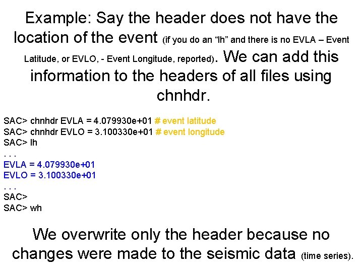
Example: Say the header does not have the location of the event (if you do an “lh” and there is no EVLA – Event Latitude, or EVLO, - Event Longitude, reported). We can add this information to the headers of all files using chnhdr. SAC> chnhdr EVLA = 4. 079930 e+01 # event latitude SAC> chnhdr EVLO = 3. 100330 e+01 # event longitude SAC> lh. . . EVLA = 4. 079930 e+01 EVLO = 3. 100330 e+01. . . SAC> wh We overwrite only the header because no changes were made to the seismic data (time series).

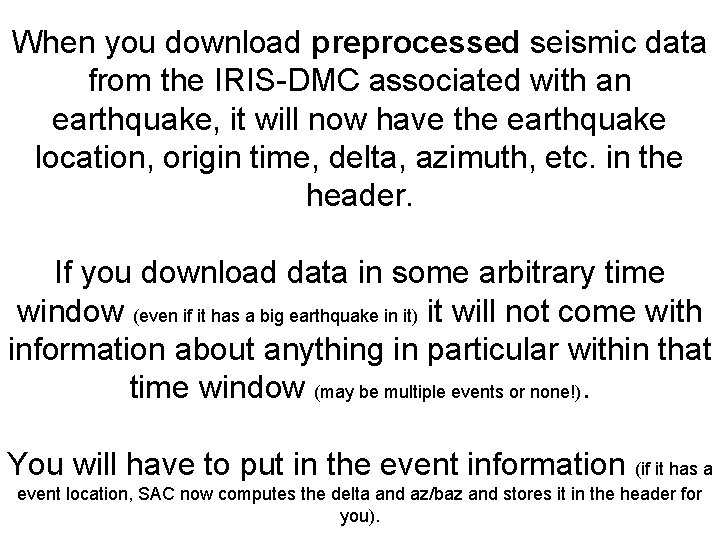
When you download preprocessed seismic data from the IRIS-DMC associated with an earthquake, it will now have the earthquake location, origin time, delta, azimuth, etc. in the header. If you download data in some arbitrary time window (even if it has a big earthquake in it) it will not come with information about anything in particular within that time window (may be multiple events or none!). You will have to put in the event information (if it has a event location, SAC now computes the delta and az/baz and stores it in the header for you).

Lining files up in time Before synch FILE: ccm_sumatra_. bhe – 1 NPTS = 389396 B = 0. 000000 e+00 KZDATE = DEC 26 (361), 2004 KZTIME = 01: 09: 52. 684 FILE: ccm_sumatra_. bhn – 2 NPTS = 389328 B = 0. 000000 e+00 KZDATE = DEC 26 (361), 2004 KZTIME = 01: 09: 48. 485 FILE: ccm_sumatra_. bhz – 3 NPTS = 389600 B = 0. 000000 e+00 KZDATE = DEC 26 (361), 2004 KZTIME = 01: 09: 43. 684 After synch B = 0. 000000 e+00 KZDATE = DEC 26 (361), 2004 KZTIME = 01: 09: 52. 684 B = -4. 199000 e+00 KZDATE = DEC 26 (361), 2004 KZTIME = 01: 09: 52. 684 B = -9. 000000 e+00 KZDATE = DEC 26 (361), 2004 KZTIME = 01: 09: 52. 684

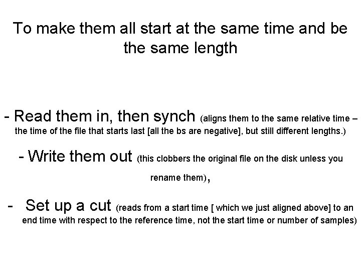
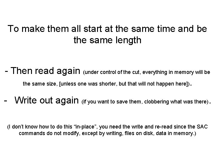
To make them all start at the same time and be the same length - Read them in, then synch (aligns them to the same relative time – the time of the file that starts last [all the bs are negative], but still different lengths. ) - Write them out (this clobbers the original file on the disk unless you rename them), - Set up a cut (reads from a start time [ which we just aligned above] to an end time with respect to the reference time, not the start time or number of samples)

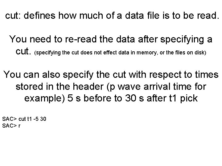
cut: defines how much of a data file is to be read. You need to re-read the data after specifying a cut. (specifying the cut does not effect data in memory, or the files on disk) You can also specify the cut with respect to times stored in the header (p wave arrival time for example) 5 s before to 30 s after t 1 pick SAC> cut t 1 -5 30 SAC> r

To make them all start at the same time and be the same length - Then read again (under control of the cut, everything in memory will be the same size, [unless one was shorter, but that will not happen here]). - Write out again (if you want to save them, clobbering what was there). (I don’t know how to do this “in-place”, you need the write and re-read since the SAC commands do not modify, except by writing, files on disk, data in memory. )

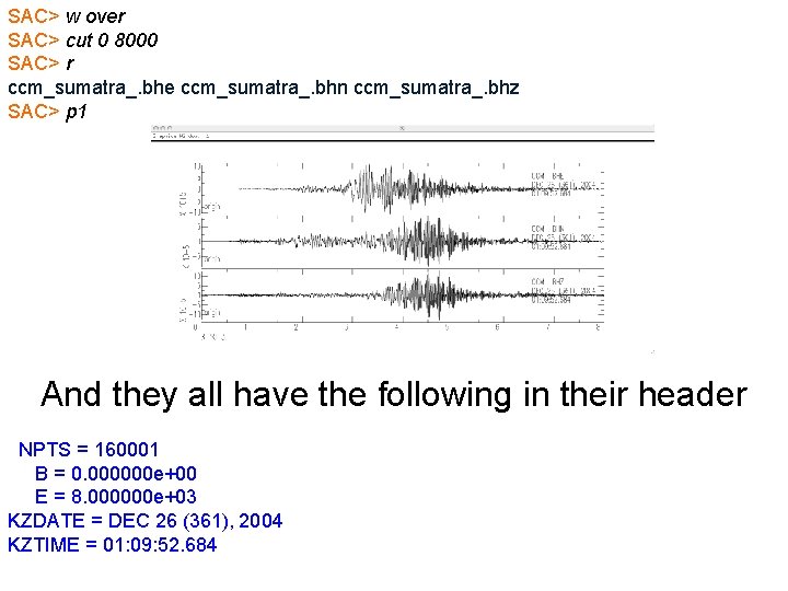
SAC> w over SAC> cut 0 8000 SAC> r ccm_sumatra_. bhe ccm_sumatra_. bhn ccm_sumatra_. bhz SAC> p 1 And they all have the following in their header NPTS = 160001 B = 0. 000000 e+00 E = 8. 000000 e+03 KZDATE = DEC 26 (361), 2004 KZTIME = 01: 09: 52. 684

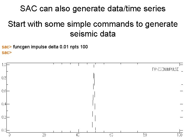
SAC can also generate data/time series Start with some simple commands to generate seismic data sac> funcgen impulse delta 0. 01 npts 100 sac>

Can generate a number of basic signals SAC> help funcgen FUNCGEN +++++++ SUMMARY ------Generates a function and stores it in memory. SYNTAX ----- ``FUNCGEN {type}, {DELTA v}, {NPTS n}, {BEGIN v}`` where type is one of the following: ``IMPULSE`` ``STEP`` ``BOXCAR`` ``TRIANGLE`` ``SINE {v 1 v 2}`` ``LINE {v 1 v 2}`` ``QUADRATIC {v 1 v 2 v 3}`` ``CUBIC {v 1 v 2 v 3 v 4}`` ``SEISMOGRAM`` ``RANDOM {v 1 v 2}`` ``IMPSTRIN {n 1 n 2. . . n. N}`` INPUT …… for many pages

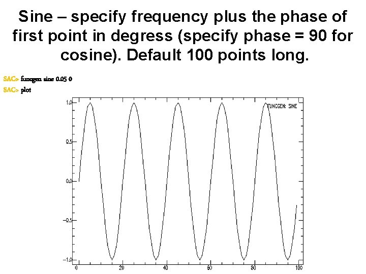
Sine – specify frequency plus the phase of first point in degress (specify phase = 90 for cosine). Default 100 points long. SAC> funcgen sine 0. 05 0 SAC> plot

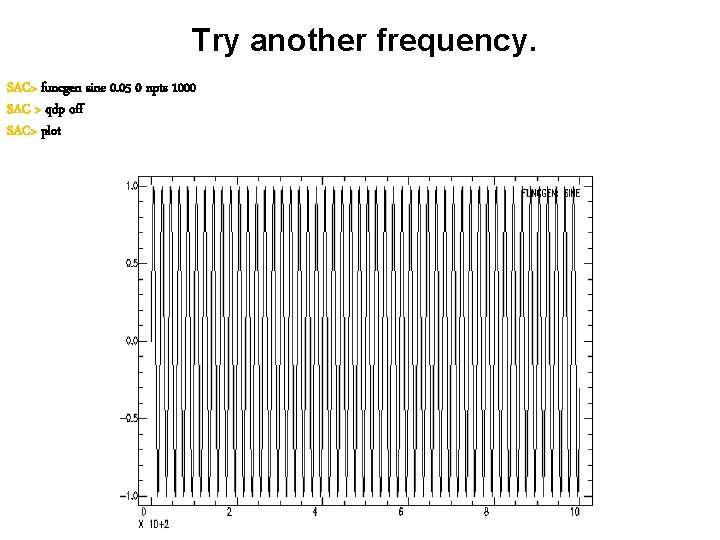
Try another frequency. SAC> funcgen sine 0. 05 0 npts 1000 SAC > qdp off SAC> plot

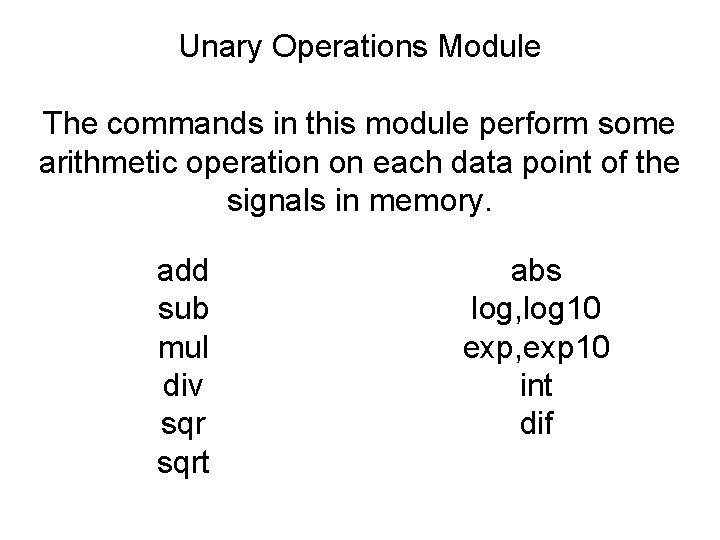
Unary Operations Module The commands in this module perform some arithmetic operation on each data point of the signals in memory. add sub mul div sqrt abs log, log 10 exp, exp 10 int dif

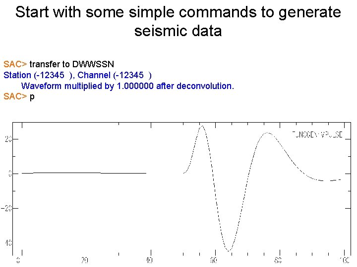
Start with some simple commands to generate seismic data SAC> transfer to DWWSSN Station (-12345 ), Channel (-12345 ) Waveform multiplied by 1. 000000 after deconvolution. SAC> p

Binary Operations Module The commands in this module perform some arithmetic operation on all the data in memory with an input file. Super clunky legacy problem from the days of computers with limited power. addf subf mulf divf merge bnoperr

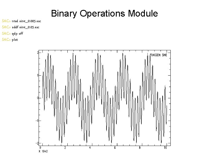
SAC> read sine_0. 005. sac SAC> addf sine_0. 05. sac SAC> qdp off SAC> plot Binary Operations Module

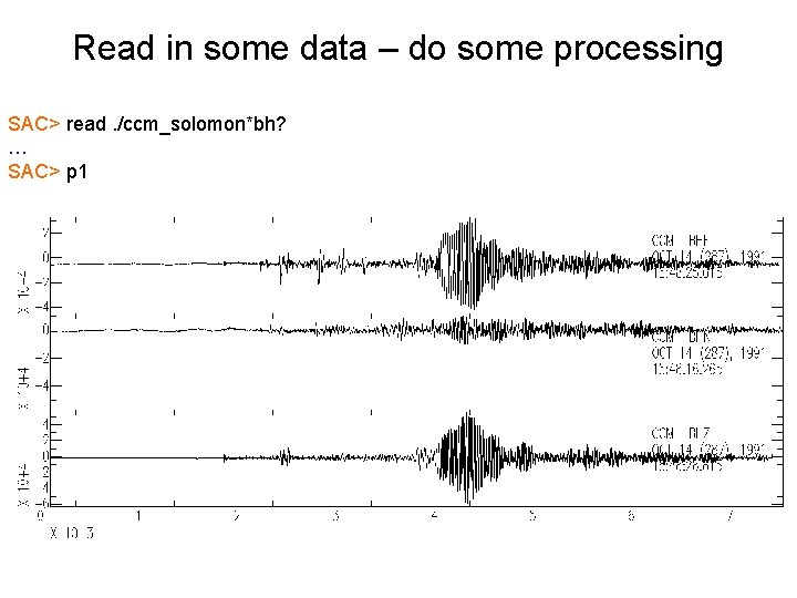
Read in some data – do some processing SAC> read. /ccm_solomon*bh? … SAC> p 1

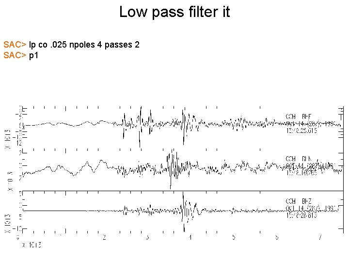
Low pass filter it SAC> lp co. 025 npoles 4 passes 2 SAC> p 1

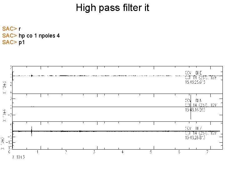
High pass filter it SAC> r SAC> hp co 1 npoles 4 SAC> p 1

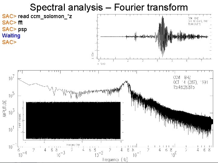
Spectral analysis – Fourier transform SAC> read ccm_solomon_*z SAC> fft SAC> psp Waiting SAC>

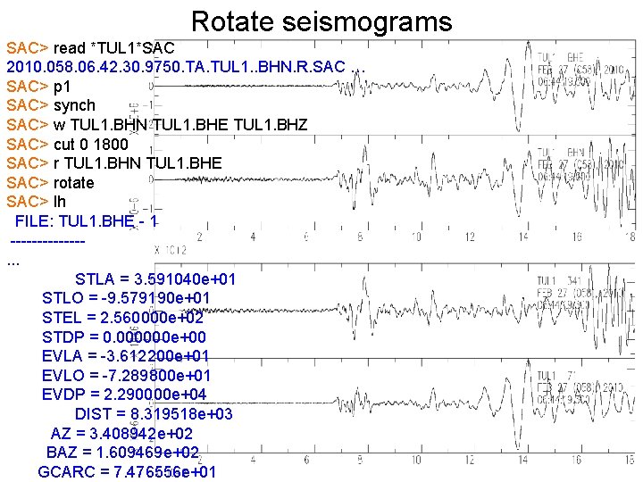
Rotate seismograms SAC> read *TUL 1*SAC 2010. 058. 06. 42. 30. 9750. TA. TUL 1. . BHN. R. SAC … SAC> p 1 SAC> synch SAC> w TUL 1. BHN TUL 1. BHE TUL 1. BHZ SAC> cut 0 1800 SAC> r TUL 1. BHN TUL 1. BHE SAC> rotate SAC> lh FILE: TUL 1. BHE - 1 -------. . . STLA = 3. 591040 e+01 STLO = -9. 579190 e+01 STEL = 2. 560000 e+02 STDP = 0. 000000 e+00 EVLA = -3. 612200 e+01 EVLO = -7. 289800 e+01 EVDP = 2. 290000 e+04 DIST = 8. 319518 e+03 AZ = 3. 408942 e+02 BAZ = 1. 609469 e+02 GCARC = 7. 476556 e+01

SAC> read TUL 1. BH[NE] TUL 1. BHE TUL 1. BHN SAC> rotate Plots R, T, Z SAC> p 1 SAC> write TUL 1. BHR TUL 1. BHT SAC> read TUL 1. BH[TR] TUL 1. BHR TUL 1. BHT SAC> read more TUL 1. BHZ Also plots R, T, Z (alphabetical order) – want R and Z together SAC> read TUL 1. BHT SAC> read more TUL 1. BHR SAC> read more TUL 1. BHZ SAC> p 1 SAC> read TUL 1. BHT TUL 1. BHR SAC> read more TUL 1. BHZ SAC> p 1 Both these work. Can now see surface waves are separated by their polarization – radial and transverse. Love wave Transverse Rayleigh wave Radial