ANALYSIS AND DESIGN OF ALGORITHMS UNITIII CHAPTER 7

ANALYSIS AND DESIGN OF ALGORITHMS UNIT-III CHAPTER 7: SPACE AND TIME TRADEOFFS 1

OUTLINE v Space and Time Tradeoffs Ø Sorting by Counting Ø Input Enhancement in String Matching § Ø Horspool’s Algorithm Hashing § § Open Hashing (Separate Chaining) Closed Hashing (Open Addressing) 2

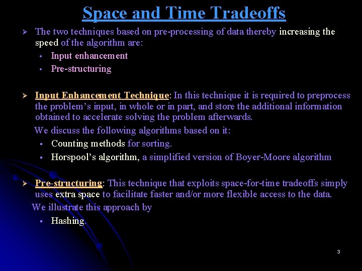
Space and Time Tradeoffs Ø The two techniques based on pre-processing of data thereby increasing the speed of the algorithm are: • Input enhancement • Pre-structuring Ø Input Enhancement Technique: In this technique it is required to preprocess the problem’s input, in whole or in part, and store the additional information obtained to accelerate solving the problem afterwards. We discuss the following algorithms based on it: § Counting methods for sorting. § Horspool’s algorithm, a simplified version of Boyer-Moore algorithm Ø Pre-structuring: This technique that exploits space-for-time tradeoffs simply uses extra space to facilitate faster and/or more flexible access to the data. We illustrate this approach by § Hashing. 3

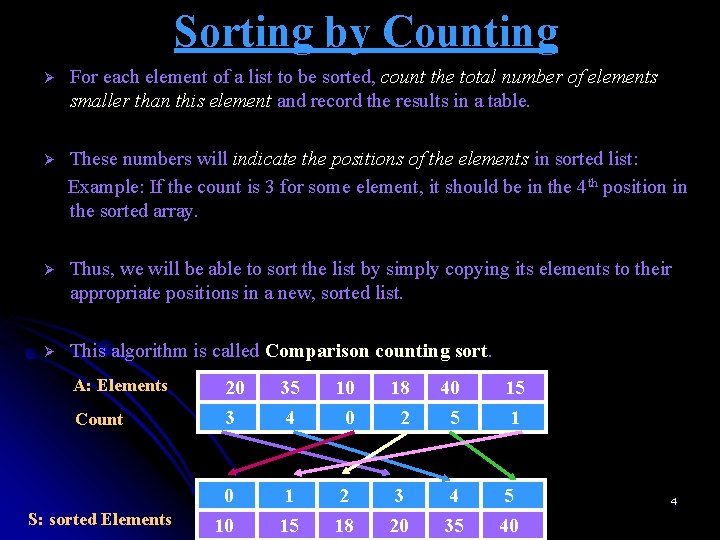
Sorting by Counting Ø For each element of a list to be sorted, count the total number of elements smaller than this element and record the results in a table. Ø These numbers will indicate the positions of the elements in sorted list: Example: If the count is 3 for some element, it should be in the 4 th position in the sorted array. Ø Thus, we will be able to sort the list by simply copying its elements to their appropriate positions in a new, sorted list. Ø This algorithm is called Comparison counting sort. A: Elements Count S: sorted Elements 20 3 0 10 35 4 10 0 18 2 40 5 15 1 1 15 2 18 3 20 4 35 5 40 4

Sorting by Counting ALGORITHM Comparison. Counting. Sort(A[0. . . n-1]) //Sorts an array by comparison counting //Input: An array A[0. . . n-1] of orderable elements //Output: Array S[0. . . n-1] of A’s elements sorted in nondecreasing order for i ← 0 to n-1 do Count[i] ← 0 for i ← 0 to n-2 do for j ← i +1 to n-1 do if A[i] < A[j] Count[j] ← Count[j] + 1 else Count[i] ← Count[i] + 1 for i ← 0 to n-1 do S[Count[i]] ← A[i] return S 5

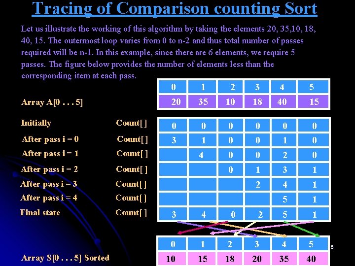
Tracing of Comparison counting Sort Let us illustrate the working of this algorithm by taking the elements 20, 35, 10, 18, 40, 15. The outermost loop varies from 0 to n-2 and thus total number of passes required will be n-1. In this example, since there are 6 elements, we require 5 passes. The figure below provides the number of elements less than the corresponding item at each pass. Array A[0. . . 5] Initially Count[ ] After pass i = 0 Count[ ] After pass i = 1 Count[ ] After pass i = 2 Count[ ] After pass i = 3 Count[ ] After pass i = 4 Count[ ] Final state Count[ ] Array S[0. . . 5] Sorted 0 20 1 35 2 10 3 18 4 40 5 15 0 3 0 1 4 0 0 0 0 1 2 3 0 0 0 1 2 4 5 1 1 3 4 0 2 5 1 0 10 1 15 2 18 3 20 4 35 5 40 6

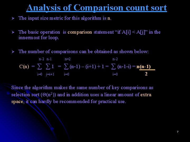
Analysis of Comparison count sort Ø The input size metric for this algorithm is n. Ø The basic operation is comparison statement “if A[i] < A[j]” in the innermost for loop. Ø The number of comparisons can be obtained as shown below: n-2 n-1 C(n) = n=2 n-2 ∑ ∑ 1 = ∑ (n-1) – (i+1) + 1 = ∑ (n-1 -i) = n(n-1) i=0 j=i+1 i=0 2 Since the algorithm makes the same number of key comparisons as selection sort (Θ(n 2)) and in addition uses a linear amount of extra space, it can hardly be recommended for practical use. 7

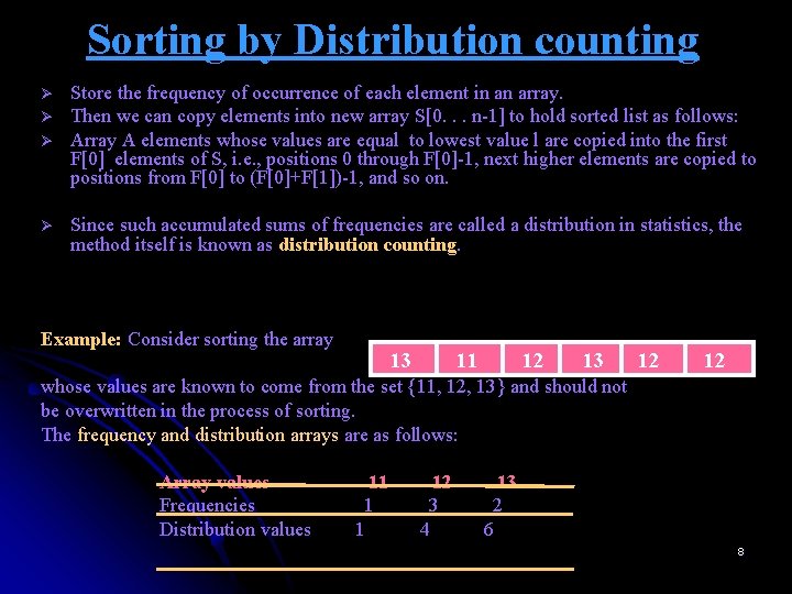
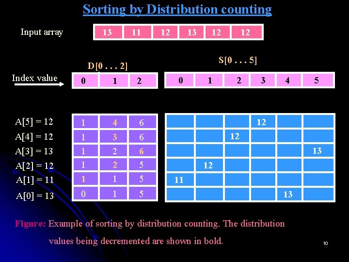
Sorting by Distribution counting Ø Ø Store the frequency of occurrence of each element in an array. Then we can copy elements into new array S[0. . . n-1] to hold sorted list as follows: Array A elements whose values are equal to lowest value l are copied into the first F[0] elements of S, i. e. , positions 0 through F[0]-1, next higher elements are copied to positions from F[0] to (F[0]+F[1])-1, and so on. Since such accumulated sums of frequencies are called a distribution in statistics, the method itself is known as distribution counting. Example: Consider sorting the array 13 11 12 13 12 12 whose values are known to come from the set {11, 12, 13} and should not be overwritten in the process of sorting. The frequency and distribution arrays are as follows: Array values Frequencies Distribution values 11 1 1 12 3 4 13 2 6 8

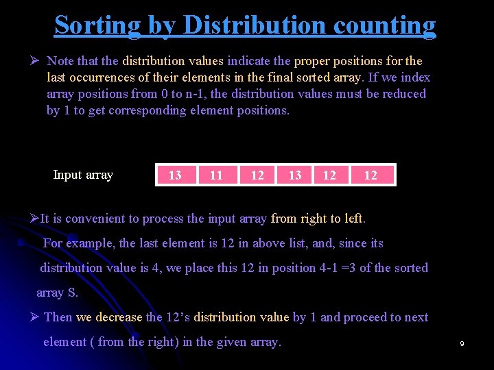
Sorting by Distribution counting Ø Note that the distribution values indicate the proper positions for the last occurrences of their elements in the final sorted array. If we index array positions from 0 to n-1, the distribution values must be reduced by 1 to get corresponding element positions. Input array 13 11 12 13 12 12 ØIt is convenient to process the input array from right to left. For example, the last element is 12 in above list, and, since its distribution value is 4, we place this 12 in position 4 -1 =3 of the sorted array S. Ø Then we decrease the 12’s distribution value by 1 and proceed to next element ( from the right) in the given array. 9

Sorting by Distribution counting Input array 13 11 12 13 12 S[0. . . 5] D[0. . . 2] Index value 0 1 2 A[5] = 12 A[2] = 12 A[1] = 11 1 1 4 3 2 2 1 6 6 6 5 5 A[0] = 13 0 1 5 A[4] = 12 A[3] = 13 12 0 1 2 3 4 5 12 12 13 12 11 13 Figure: Example of sorting by distribution counting. The distribution values being decremented are shown in bold. 10

Sorting by Distribution counting ALGORITHM Distribution. Counting(A[0. . . n-1], L, U) //Sorts an array of integers from a limited range by distribution counting //Input: An array A[0. . . n-1] of integers between l and u (l ≤ u) //Output: Array S[0. . . n-1] of A’s elements sorted in nondecreasing order for j ← 0 to U – L do D[j] ← 0 //initialize frequencies for i ← 0 to n – 1 do D[A[i] – L] ← D[A[i] – L] + 1 //compute frequencies for j ← 1 to U – L do D[j] ← D[j– 1] + D[j] //reuse for distribution for i ← n-1 downto 0 do j ← A[i] – L S[D[j] – 1] ← A[i] D[j] ← D[j] – 1 13 11 12 13 12 12 return S 11

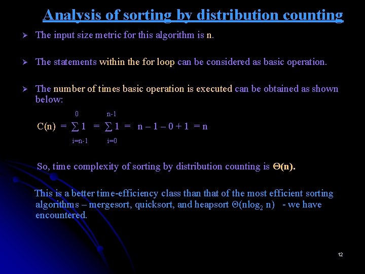
Analysis of sorting by distribution counting Ø The input size metric for this algorithm is n. Ø The statements within the for loop can be considered as basic operation. Ø The number of times basic operation is executed can be obtained as shown below: 0 n-1 C(n) = ∑ 1 = n – 1 – 0 + 1 = n i=n-1 i=0 So, time complexity of sorting by distribution counting is Θ(n). This is a better time-efficiency class than that of the most efficient sorting algorithms – mergesort, quicksort, and heapsort Θ(nlog 2 n) - we have encountered. 12

Input Enhancement in String Matching Ø The pattern matching algorithm using Brute-force method had the worst-case efficiency of Θ(mn) where m is the length of the pattern and n is the length of the text. In the average-case, its efficiency turns out to be in Θ(n). Ø Several better algorithms have been discovered. Most of them exploit the input enhancement idea: preprocess the pattern to get some information about it, store this information in a table, and then use this information during an actual search for the pattern in a given text. Ø The various algorithms which uses the input enhancement technique for string matching are: § Knuth-Morris-Pratt algorithm § Boyer-Moore algorithm § Horspool’s algorithm which is a simplified version of Boyer Moore algorithm. 13

Horspool’s Algorithm A simplified version of Boyer-Moore algorithm: Ø preprocesses pattern to generate a shift table that determines how much to shift the pattern when a mismatch occurs Ø Determines the size of shift by looking at the character c of the text that was aligned against the last character of the pattern. 14

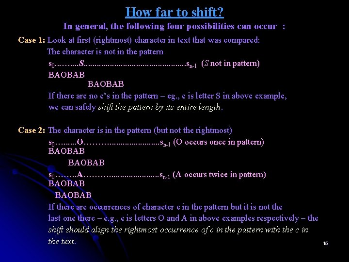
How far to shift? In general, the following four possibilities can occur : Case 1: Look at first (rightmost) character in text that was compared: The character is not in the pattern s 0. . . …. . S. . . sn-1 (S not in pattern) BAOBAB If there are no c’s in the pattern – eg. , c is letter S in above example, we can safely shift the pattern by its entire length. Case 2: The character is in the pattern (but not the rightmost) s 0…. . . O………. . . sn-1 (O occurs once in pattern) BAOBAB s 0……. . A………. . . sn-1 (A occurs twice in pattern) BAOBAB If there are occurrences of character c in the pattern but it is not the last one there – e. g. , c is letters O and A in above examples respectively – the shift should align the rightmost occurrence of c in the pattern with the c in the text. 15

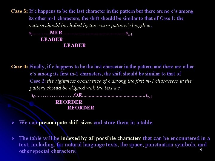
Case 3: If c happens to be the last character in the pattern but there are no c’s among its other m-1 characters, the shift should be similar to that of Case 1: the pattern should be shifted by the entire pattern’s length m. s 0. . . ……. . MER. . . sn-1 LEADER Case 4: Finally, if c happens to be the last character in the pattern and there are other c’s among its first m-1 characters, the shift should be similar to that of Case 2: the rightmost occurrence of c among the first m-1 characters in the pattern should be aligned with the text’s c. s 0. . . ………………. . OR. . . sn-1 REORDER Ø We can precompute shift sizes and store them in a table. Ø The table will be indexed by all possible characters that can be encountered in a text, including, for natural language texts, the space, punctuation symbols, and 16 other special characters.

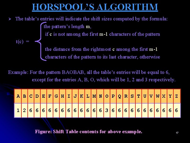
HORSPOOL’S ALGORITHM Ø The table’s entries will indicate the shift sizes computed by the formula: the pattern’s length m, if c is not among the first m-1 characters of the pattern t(c) = the distance from the rightmost c among the first m-1 characters of the pattern to its last character, otherwise Example: For the pattern BAOBAB, all the table’s entries will be equal to 6, except for the entries A, B, O, which will be 1, 2 and 3 respectively. A B C D E F G H I J K L M N O P Q R S T U V W X Y Z 1 2 6 6 6 3 6 6 6 Figure: Shift Table contents for above example. 17

ALGORITHM FOR COMPUTING THE SHIFT TABLE ENTRIES ALGORITHM Shift. Table(P[0. . . m-1]) //Fills the shift table used by Horspool’s algorithm //Input: Pattern P[0. . . m-1] and an alphabet of possible characters //Output: Table[0. . . size-1] indexed by the alphabet’s characters and // filled with shift sizes computed initialize all the elements of Table with m for j ← 0 to m-2 do Table[P[j]] ← m – 1 – j return Table Ø Ø Initialize all the entries to the pattern’s length m. Scan the pattern left to right repeating the following step m-1 times: for the jth character of pattern (0 ≤ j ≤ m-2), overwrite its entry in the table with m-1 -j, which is the character’s distance to the right end of the pattern. Since algorithm scans pattern from left to right, the last overwrite will happen for a character’s rightmost occurrence. 18

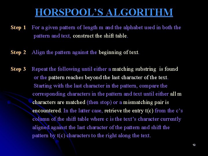
HORSPOOL’S ALGORITHM Step 1 For a given pattern of length m and the alphabet used in both the pattern and text, construct the shift table. Step 2 Align the pattern against the beginning of text. Step 3 Repeat the following until either a matching substring is found or the pattern reaches beyond the last character of the text. Starting with the last character in the pattern, compare the corresponding characters in the pattern and text until either all m characters are matched (then stop) or a mismatching pair is encountered. In the latter case, retrieve the entry t(c) from the c’s column of the shift table where c is the text’s character currently aligned against the last character of the pattern and shift the pattern by t(c) characters to the right along the text. 19

HORSPOOL’S ALGORITHM Horspool. Matching(P[0…m-1], T[0…n-1]) //Implements Horspool’s algorithm for string matching //Input: Pattern P[0…m-1] and T[0…n-1] //Output: The index of the left end of the first matching substring or //-1 if there are no matches Shift. Table(P[0…m-1]) // generate Table of shifts i ← m-1 // position of the pattern’s right end while i ≤ n-1 do k ← 0 //number of matched characters while k ≤ m-1 and P[m – 1 - k] = T[i - k] do k← k+1 if k = m return i – m + 1 else i ← i + Table[T[i]] return -1 20

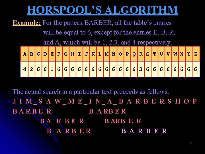
HORSPOOL’S ALGORITHM Example: For the pattern BARBER, all the table’s entries will be equal to 6, except for the entries E, B, R, and A, which will be 1, 2, 3, and 4 respectively. A B C D E F G H I J K L M N O P Q R S T U V W X Y Z 4 2 6 6 1 6 6 6 3 6 6 6 6 The actual search in a particular text proceeds as follows: J I M_S A W_M E_I N_A_B A R B E R S H O P BARBE R B A RB E R BA R BE R B ARB E R B A RB ER B A R B E R 21

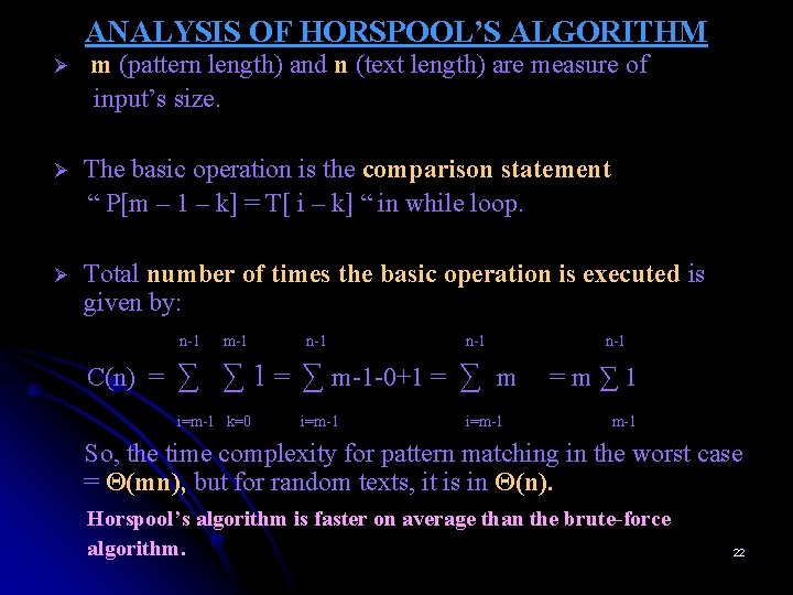
ANALYSIS OF HORSPOOL’S ALGORITHM Ø m (pattern length) and n (text length) are measure of input’s size. Ø The basic operation is the comparison statement “ P[m – 1 – k] = T[ i – k] “ in while loop. Ø Total number of times the basic operation is executed is given by: n-1 m-1 n-1 C(n) = ∑ ∑ 1 = ∑ m-1 -0+1 = ∑ m i=m-1 k=0 i=m-1 n-1 =m∑ 1 m-1 So, the time complexity for pattern matching in the worst case = Θ(mn), but for random texts, it is in Θ(n). Horspool’s algorithm is faster on average than the brute-force algorithm. 22

Hashing Ø A very efficient method for implementing a dictionary, i. e. , a set with the operations: l search l insert l delete Ø Based on representation-change and space-for-time tradeoff ideas Ø Important applications: l symbol tables – a table of computer program symbols generated during compilation. l databases –hashing is useful for storing very large dictionaries on disks; this variation of hashing is called extendible hashing. 23

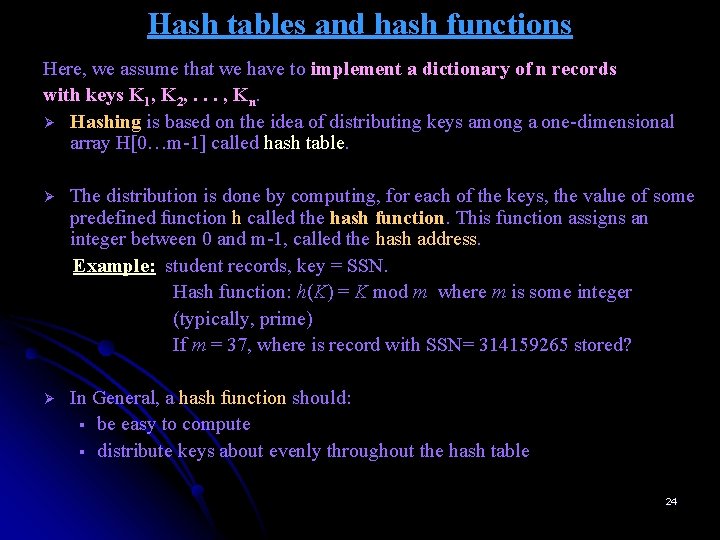
Hash tables and hash functions Here, we assume that we have to implement a dictionary of n records with keys K 1, K 2, . . . , Kn. Ø Hashing is based on the idea of distributing keys among a one-dimensional array H[0…m-1] called hash table. Ø The distribution is done by computing, for each of the keys, the value of some predefined function h called the hash function. This function assigns an integer between 0 and m-1, called the hash address. Example: student records, key = SSN. Hash function: h(K) = K mod m where m is some integer (typically, prime) If m = 37, where is record with SSN= 314159265 stored? Ø In General, a hash function should: § be easy to compute § distribute keys about evenly throughout the hash table 24

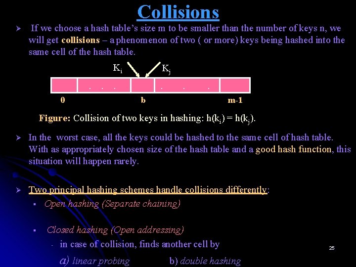
Collisions Ø If we choose a hash table’s size m to be smaller than the number of keys n, we will get collisions – a phenomenon of two ( or more) keys being hashed into the same cell of the hash table. . . Ki Kj . . 0 . . b m-1 Figure: Collision of two keys in hashing: h(ki) = h(kj). Ø In the worst case, all the keys could be hashed to the same cell of hash table. With as appropriately chosen size of the hash table and a good hash function, this situation will happen rarely. Ø Two principal hashing schemes handle collisions differently: § Open hashing (Separate chaining) § Closed hashing (Open addressing) - in case of collision, finds another cell by a) linear probing b) double hashing 25

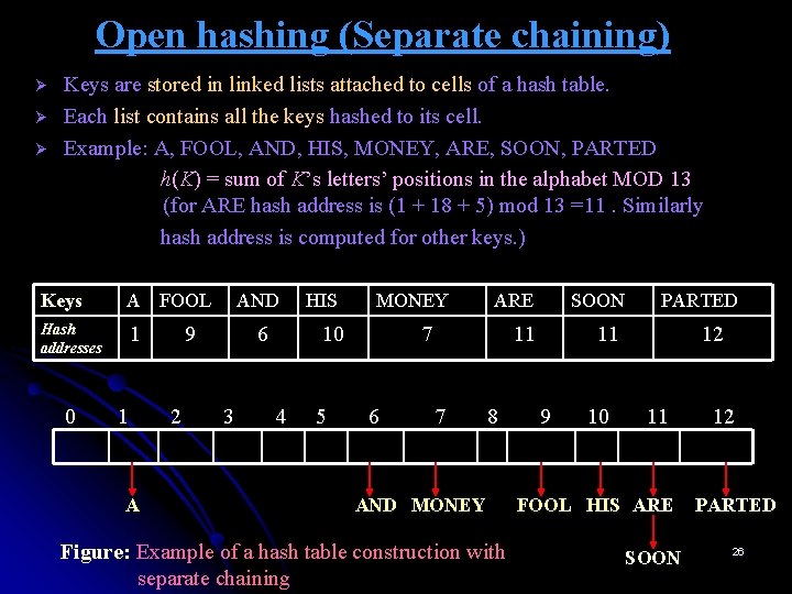
Open hashing (Separate chaining) Ø Ø Ø Keys are stored in linked lists attached to cells of a hash table. Each list contains all the keys hashed to its cell. Example: A, FOOL, AND, HIS, MONEY, ARE, SOON, PARTED h(K) = sum of K’s letters’ positions in the alphabet MOD 13 (for ARE hash address is (1 + 18 + 5) mod 13 =11. Similarly hash address is computed for other keys. ) Keys A FOOL Hash addresses 1 0 1 A AND 9 2 6 3 HIS MONEY 10 4 5 ARE SOON 11 11 7 6 7 8 AND MONEY Figure: Example of a hash table construction with separate chaining 9 10 PARTED 12 11 FOOL HIS ARE SOON 12 PARTED 26

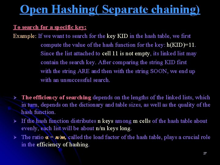
Open Hashing( Separate chaining) To search for a specific key: Example: If we want to search for the key KID in the hash table, we first compute the value of the hash function for the key: h(KID)=11. Since the list attached to cell 11 is not empty, its linked list may contain the search key. After comparing the string KID first with the string ARE and then with the string SOON, we end up with an unsuccessful search. Ø Ø Ø The efficiency of searching depends on the lengths of the linked lists, which in turn, depends on the dictionary and table sizes, as well as the quality of the hash function. If the hash function distributes n keys among m cells of the hash table about evenly, each list will be about n/m keys long. The ratio α = n/m, called the load factor of the hash table, plays a crucial role in the efficiency of hashing. 27

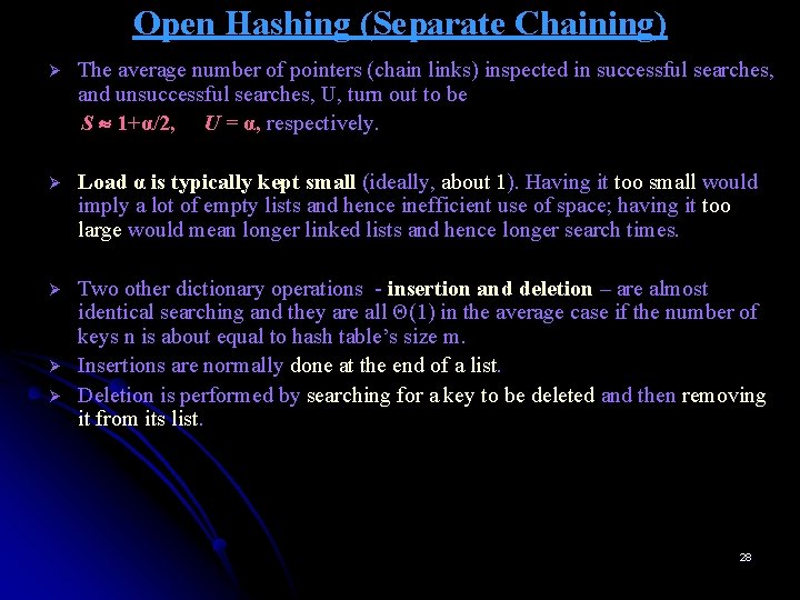
Open Hashing (Separate Chaining) Ø The average number of pointers (chain links) inspected in successful searches, and unsuccessful searches, U, turn out to be S 1+α/2, U = α, respectively. Ø Load α is typically kept small (ideally, about 1). Having it too small would imply a lot of empty lists and hence inefficient use of space; having it too large would mean longer linked lists and hence longer search times. Ø Two other dictionary operations - insertion and deletion – are almost identical searching and they are all Θ(1) in the average case if the number of keys n is about equal to hash table’s size m. Insertions are normally done at the end of a list. Deletion is performed by searching for a key to be deleted and then removing it from its list. Ø Ø 28

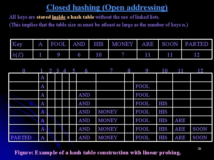
Closed hashing (Open addressing) All keys are stored inside a hash table without the use of linked lists. (This implies that the table size m must be atleast as large as the number of keys n. ) Key A FOOL AND HIS MONEY ARE SOON PARTED h(K) 1 9 6 10 7 11 11 12 1 2 3 4 0 5 6 7 8 9 10 11 12 A A PARTED FOOL A AND FOOL HIS A AND MONEY FOOL HIS ARE SOON Figure: Example of a hash table construction with linear probing. 29

Closed Hashing (Open Addressing) Ø Different strategies can be employed for collision resolution. v Linear probing: This strategy checks the cell following the one where the collision occurs. If that cell is empty, the new key is installed there; if the next cell is already occupied, the availability of that cell’s immediate successor is checked, and so on. Note that if the end of the hash table is reached, the search is wrapped to the beginning of the table; i. e, it is treated as a circular array. o To search for a given key K, we start by computing h(k) where h is the hash function used in the table’s construction. If the cell h(k) is empty, the search is unsuccessful. If the cell is not empty, we must compare K with the cell’s occupant: if they are equal, we have found a matching key; if they are not, we compare K with a key in the next cell and continue in this manner until we encounter either a matching key (a successful search) or an empty cell (unsuccessful search). 30

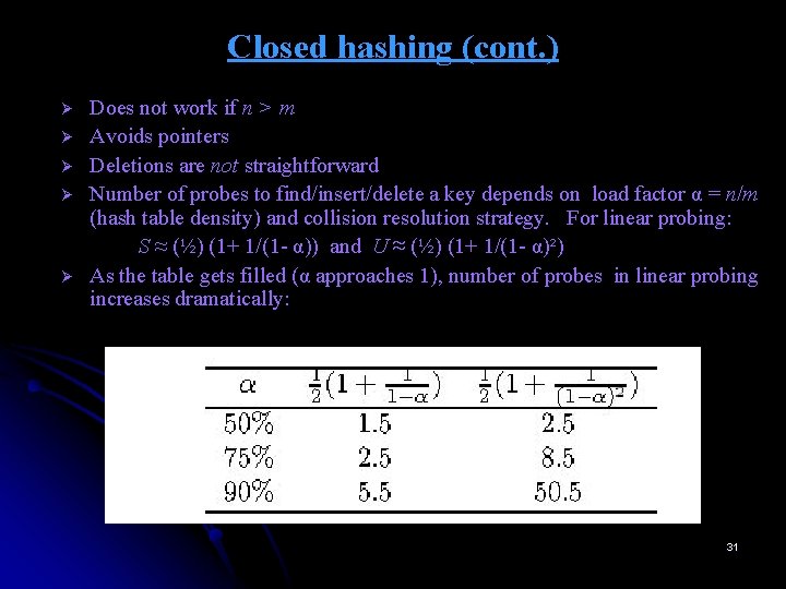
Closed hashing (cont. ) Ø Ø Ø Does not work if n > m Avoids pointers Deletions are not straightforward Number of probes to find/insert/delete a key depends on load factor α = n/m (hash table density) and collision resolution strategy. For linear probing: S ≈ (½) (1+ 1/(1 - α)) and U ≈ (½) (1+ 1/(1 - α)²) As the table gets filled (α approaches 1), number of probes in linear probing increases dramatically: 31

End of Chapter 7 32