An Overview of Numerical Weather Prediction Models Overview

An Overview of Numerical Weather Prediction Models

Overview • What is a Numerical Forecast Model • Models: The Good, Bad, and Ugly – Increasing awareness and understanding of models and how they work • The Importance of Using Forecast Models only as a Tool. • Model Behavior and Verification: Actual studies of model performance

Where is Hurricane Georges Going? Model Forecasts

Where is Hurricane Georges Going? Model Forecasts

Georges Went Here Instead!

Lesson from this Exercise • Numerical model forecasts are not a panacea. • Experienced and alert forecasters/analysts may add significant value to numerical weather forecasts. • Forecasters must have a basic understanding of model interpretation, biases and limitations in different forecasting situations before they can accurately deviate from model forecasts. • Model interpretation needs to be rooted a solid knowledge of meteorological theory and model structure.

Operational Model Overviews • Models are either regional or global • Regional Models Model – LFM – NGM – ETA – RUC – MM 5 – GFDL – COAMPS – WRF Owner (NCEP) (Phased out) (NCEP) (Replaced by NAM, NAM-WRF) (NCAR/NCEP) (Replaced by RAP) (PSU / Air Force, etc…. ) (NCEP and GFDL Lab) (Navy) (NCEP)

Operational Model Overviews • Global Models Model Owner – GFS (Formerly the AVN/MRF) (NCEP) – NOGAPS – GEM – ECMWF – UKMET (Navy) (Canada) (European Union) (United Kingdom)

What is the Fundamental Difference Between Grid Point and Spectral Models? • Grid point and spectral models are based on the same set of primitive equations. However, each type formulates and solves the equations differently. The differences in the basic mathematical formulations contribute to different characteristic errors in model guidance. The differences in the basic mathematical formulations lead to different methods for representing data. Grid point models represent data at discrete, fixed grid points, whereas spectral models use continuous wave functions. Different types and amounts of errors are introduced into the analyses and forecasts due to these differences in data representation. The characteristics of each model type along with the physical and dynamic approximations in the equations influence the type and scale of features that a model may be able to resolve.

What is a Numerical Forecast Model? (i. e. , First Guess)

Model Components • Numerical Models consist of multiple parts. • The actual “forecasting” part of the model is only one part of a very complicated procedure of – – data collection and assimilation Forecasting Post Processing Distribution to users

Caution! There are many sources of possible error in an NWP forecast!!!

Sources of Model Error

Data Assimilation • Data assimilation is the process through which real world observations enter the model's forecast cycles • Provide a safeguard against model error growth • Contribute to the initial conditions for the next model run

DATA • The goal of the DA system is to provide a reality check for the short-term model forecast used to start up the current forecast cycle.

Observation Increment • How does DA make observations comparable to the first guess? • How can observations made at different times, with different patterns of coverage and sampling characteristics, all be combined into one analysis? • Why does good data sometimes get rejected in the process? • How can observations, providing a reality check, be combined with crucial structure information in the model short-range forecast?

Analysis • • Using Observation Increments to Make the Analysis Problems from the Start Heart of Analysis: How Much to Weight Observations Versus the Forecast Balancing Observations Versus the Forecast Assumptions Affecting the Analysis Why Some Data Types Are Not as Useful as Others Including the Data Rejection Process in the Analysis Stage ("Nonlinear QC") Tuning

Operational Tips • Judging Analysis Quality • Compensating for a Bad Analysis: History of Data Void • Compensating for a Bad Analysis: Bad First Guess • Compensating for a Bad Analysis: Good Data Rejected • Compensating for a Bad Analysis: Analysis • Assumptions Violated • Compensating for a Bad Analysis: Tuning

Observational Data Coverage Surface Observations

Observational Data Coverage Surface Observations

Observational Data Coverage Weather Buoys

Observational Data Coverage Conus Rawinsonde Network

Observational Data Coverage Oceanic Rawinsonde Network

Observational Data Coverage Satellite-Derived Winds

Errors in Data and Quality Control • Instrument Errors • Representativeness Errors – vertical, horizontal, and temporal • Converting remotely-sensed data into high-quality observations which can be appropriately integrated with other data. – Satellite data must be constantly “calibrated” by rawinsonde data for constantly changing atmospheric environments. (What happens in regions void of rawinsondes? )

Errors in Data and Quality Control Bogus Lows

Errors in Objective Analysis H

Errors in Objective Analysis Underground

Errors in Data Assimilation

Errors in Data Assimilation

Model Initialization Problems · Model first guess · · can sometimes overwhelm actual data First guess may result in observations being ignored In this case, Hurricane Earl incorrectly analyzed several hundred miles too far SW of its actual position (From COMET)

Poor Analysis = Huge Forecast Errors · Initial placement · of a few hundred miles translated to a nearly 1, 000 mile error by 48 -h forecast Such errors can disrupt the larger-scale pattern (From COMET)

Ways to Check the Quality of Model Analyses • Use observations, local area workcharts, radar, and satellite to check the quality of the model analyses • Compare different model analyses to each other. • Look for dynamic consistency between model levels • Read the Model Diagnostic Discussion at HPC – http: //www. hpc. ncep. noaa. gov/html/about_model_diag. shtml – http: //www. hpc. ncep. noaa. gov/html/discuss. shtml

Atmospheric Variables Not Routinely Measured • • • Longwave and Shortwave Radiation Cloud Water and Ice Content Vertical Motion Surface roughness of the ocean (i. e. , waves) Turbulence Many more…. .

The Power of the First Guess • The first guess (an earlier 6 or 12 hour forecast) is the model’s initial impression of the atmosphere’s current condition. • The first guess is innocent until proven guilty. • The first guess is most easily modified in datarich areas (i. e. , CONUS) • The first guess is least easily modified in data poor areas (i. e. oceans, etc…)

Ways to Check the First Guess Influence on the Analysis • Overlay observations on the model analysis • Compare hand-analyzed workcharts and alternate local computer-generated analyses to the model analysis. • Remember that your local computer-generated analyses (without a gridded background field) are totally blind except for the observations you feed them. Use with caution!

Ways to Check the First Guess Influence on the Analysis • Compare different model analyses to each other.

Ways to Check the First Guess Influence on the Analysis • Compare model analyses to satellite, radar, and other real-time information. • These are important functions all forecasters should routinely perform. It is one of the most powerful ways a forecaster can add value to the model guidance!- especially for short-range forecasts.

Errors in the Model • Equations of Motion are Incomplete – Massive simplifications (i. e. , parameterizations) are necessary to make the model work. • Errors in the Numerical Approximation – Horizontal and Vertical Resolution – Time integration procedure • Boundary Conditions – Horizontal and Vertical boundaries

Horizontal Resolution • The horizontal resolution of an NWP model is related to the spacing between grid points for grid point models or the number of waves that can be resolved for spectral models. • 'Resolution' is defined here in terms of the grid spacing or wave number and represents the average area depicted by each grid point in a grid point model or the number of waves used in a spectral model. • Note that the smallest features that can be accurately represented by a model are many times larger than the grid 'resolution. ' In fact, phenomena with dimensions on the same scale as the grid spacing are unlikely to be depicted or predicted within a model.

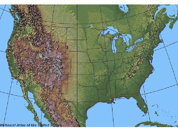
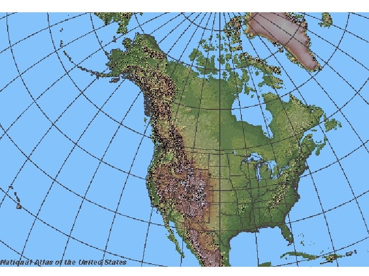
Horizontal Resolution From: COMET: http: //meted. ucar. edu/nwp/pcu 1/ic 2/frameset. htm (Introduction)

Horizontal Resolution (Grid) From: COMET: http: //meted. ucar. edu/nwp/pcu 1/ic 2/frameset. htm (Grid Spacing)

Horizontal Resolution (Grid) • It is important to know the amount of area between grid points, since atmospheric processes and events occurring over areas near to or smaller than this size will not be included in the model. From: COMET: http: //meted. ucar. edu/nwp/pcu 1/ic 2/frameset. htm (Grid Spacing, p 2)

Horizontal Resolution (Grid) • Grid point models can incorporate data at all resolutions, but can introduce errors by doing so. It takes about five to seven grid points to get reasonable approximations of most weather features. Still more points per wave feature are often necessary to get a good forecast.

Horizontal Resolution (LFM)

Horizontal Resolution (ETA)

Horizontal Resolution (Spectral) • In spectral models, the horizontal resolution is designated by a "T" number (for example, T 80), which indicates the number of waves used to represent the data. The "T" stands for triangular truncation, which indicates the particular set of waves used by a spectral model. • Spectral models represent data precisely out to a maximum number of waves, but omit all the more detailed information contained in smaller waves. The wavelength of the smallest wave in a spectral model is represented as: minimum wavelength = N 360 degrees where N is the total number of waves (the "T" number). From: COMET: http: //meted. ucar. edu/nwp/pcu 1/ic 2/frameset. htm (Wave No. , p 1)

Conversion of Spectral to Grid Resolution • Because spectral and grid point models preserve information in different ways, no precise equivalent grid spacing can be given for a spectral model resolution. However, we can approximate the grid spacing to obtain equivalent accuracy to a spectral model with a fixed number of waves using a very simple approach. First, we assume that three grid points are sufficient to capture the information contained in each of a series of continuous waves. The approximate grid spacing with the same accuracy as a spectral model can then be represented as From: COMET: http: //meted. ucar. edu/nwp/pcu 1/ic 2/frameset. htm (Wave No. , p 2)

Conversion of Spectral to Grid Resolution • For a T 80 model, this results in a maximum grid spacing for equivalent accuracy of about: From: COMET: http: //meted. ucar. edu/nwp/pcu 1/ic 2/frameset. htm (Wave No. , p 2)

Discussion of Horizontal Resolution between Grid-Point and Spectral Models • The dynamics of spectral models retain far better wave representation than grid point models. • However, the spectral model physics is calculated on a grid, with about three (better number is five) times as many grid lengths as number of waves used to represent the data. • Since it takes five to seven grid points to represent 'wavy' data well and even more for features that include discontinuities, the resolution of the physics is poorer than the above formulation indicates and degrades the quality of the spectral model forecast. From: COMET: http: //meted. ucar. edu/nwp/pcu 1/ic 2/frameset. htm (Wave No. , p 2)

Horizontal Resolution Summary: (Grid vs Spectral Models) • In summary, spectral models do a fine job with 'dry' waves in the free atmosphere, but have coarser representation of the physics, including surface properties. • The resulting overall forecast quality is somewhere between these two extremes and varies on a case-by -case basis. The more physics that is involved in the evolution of the forecast, the less the advantage in spectral model forecasts compared to comparable resolution grid point forecasts. From: COMET: http: //meted. ucar. edu/nwp/pcu 1/ic 2/frameset. htm (Wave No. , p 2)

Terrain • Two factors limit model representation of orography: – The horizontal resolution of the model – The horizontal resolution of the terrain dataset used • If the terrain dataset is coarse, it cannot provide details about the topography to high-resolution models. If the model cannot resolve terrain features, terrain details provided in the dataset will be averaged out. In most cases, some terrain smoothing is desirable, in part because airflow over complex terrain otherwise generates small-scale noise that can mask the larger-scale signal. From: COMET: http: //meted. ucar. edu/nwp/pcu 1/ic 2/frameset. htm (Terrain, p. 3)

NGM Topography (200 m intervals)

Vertical Resolution Comparisons

Vertical Resolution (Early ETA)

Vertical Resolution (Meso ETA)

Terrain-following Sigma Coordinates

Domain and Boundary Conditions • Model domain refers to a model's area of coverage. Limited-area models (LAMs) have horizontal (lateral) and top and bottom (vertical) boundaries, whereas global models, which by nature cover the entire earth, have only vertical boundaries. For limited-area models, larger-domain models supply the data for the lateral boundary conditions.

Errors in the Model • Terrain • Physical Processes – Precipitation • Stratiform • Convective – Radiation (short- and long-wave) – Surface energy balance – Boundary Layer – Boundary Conditions

Errors in the Model • Parameterizations: – NWP models cannot resolve weather features and/or processes that occur within a single model grid box. – These “sub-grid scale” features and processes must be parameterized in the model • Go to the following web pages:

Errors in the Model • Post processing of information – Forecast fields are interpolated, smoothed, and manipulated. The forecast panels you see may not be at the detail that the model produced. – Many products (vorticity, divergence, relative humidity, sea level pressure, etc. . . ) are derived indirectly from model forecasts of winds, temperature, moisture, and surface pressure).

Errors in the Model • Interpret forecast products carefully! Learn about what is actually being displayed. – Examples: • Surface Winds • FOUS vs MOS • Meteograms

Example of Model Forecast Error • Extremely cold, dense arctic air was forcing a shallow arctic frontal layer southward through the Plains. • The poor vertical resolution of the NGM could not resolve the correct placement of the shallow front. • The somewhat better vertical resolution of the ETA provided a more accurate forecast. • But both models had sizeable forecast errors.

Anticipate Model Derived Fields! • Example: Anticipate Vertical Motion Fields before looking at model cloud cover and precip forecasts. – Temperature Advection • Warm Advection (ascent) • Cold Advection (descent) – Vorticity Advection • PVA (lifting) • NVA (sinking) – Kinematic Wind Characteristics: • Apply the terms of the ageostrophic wind equation • Also look for upper tropospheric confluence (possible convergence) or diffluence (possible divergence)

Anticipate Model Derived Fields! – Kinematic Wind Characteristics (continued) • Surface Convergence (lifting) • Surface Divergence (sinking) – Topography • Upslope/Downslope • Coastal seabreeze/landbreeze – Thermodynamic Stability/Instability • Vertical temperature & moisture structure – Fog – Convection vs stratiform – Lake-effect precip