A PRESENTATION ON Statistical Analysis and Interpretation of

A PRESENTATION ON Statistical Analysis and Interpretation of Data Dr R N Patel Professor Mechanical Engg. Department INSTITUTE OF TECHNOLOGY NIRMA UNIVERSITY, AHMEDAMAD.

OVERVIEW 1. Analysis of experimental data 2. Causes and types of errors 3. Uncertainty analysis 4. Interpolation 5. Regression 6. Method of least square

OVERVIEW 7. Data presentation 8. Hypothesis testing 9. Z- test 10. T-test MTECH THERMAL ENGG 20010 -11

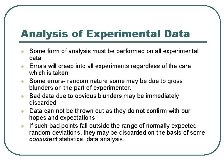
Analysis of Experimental Data l l l Some form of analysis must be performed on all experimental data Errors will creep into all experiments regardless of the care which is taken Some errors- random nature some may be due to gross blunders on the part of experimenter. Bad data due to obvious blunders may be immediately discarded Data can not be thrown out as they do not confirm with our hopes and expectations If such bad points fall outside the range of normally expected random deviations, they may be discarded on the basis of some consistent statistical data analysis.

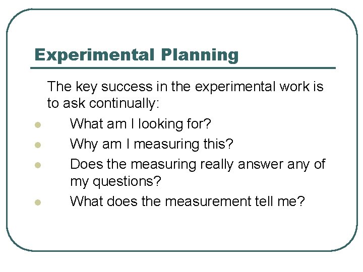
Experimental Planning l l The key success in the experimental work is to ask continually: What am I looking for? Why am I measuring this? Does the measuring really answer any of my questions? What does the measurement tell me?

Experimental Planning l l l l One should look for following in the initial phase of experimental planning What primary variables shall be investigated? What range of primary variables will be necessary to describe the phenomenon under study? How many data points shall be taken? What instrument accuracy is required? If a dynamic measurement is involved, what frequency response must the instrument have? Are the instruments commercially available? What provision is made for recording the data?

Causes and types of errors Single sample and multi sample data l Uncertainty may not be discovered by repetition in single sample data. In multi sample enough experiments are performed so that reliability of the results is assured by statistics Types of errors l Gross blunders in apparatus – which may invalidate the data, careful experimenter will be able to eliminate such errors l Fixed errors- causes repeated readings to be in error by roughly the same magnitude but for some unknown reasons l They are also called systematic errors or biased errors l Random errors- by personnel fluctuations, random electronic fluctuations in the apparatus, various influence of friction, etc l Fixed errors may sometimes be estimated by using some theoretical methods l

Uncertainty Analysis Error analysis on commonsense basis l l Uncertainty in experimental analysis is due to instrument accuracy, Competence of user, etc. Our interest is to see uncertainty in final result due to uncertainties in primary measurements. Thumb rule- uncertainty in final result is max error in any parameter used. Another common sense analysis would combine all the errors in the most detrimental way in order to calculate the max error in final result.

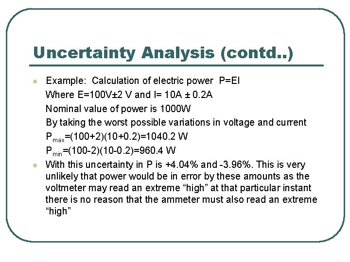
Uncertainty Analysis (contd. . ) l l Example: Calculation of electric power P=EI Where E=100 V± 2 V and I= 10 A ± 0. 2 A Nominal value of power is 1000 W By taking the worst possible variations in voltage and current Pmax=(100+2)(10+0. 2)=1040. 2 W Pmin=(100 -2)(10 -0. 2)=960. 4 W With this uncertainty in P is +4. 04% and -3. 96%. This is very unlikely that power would be in error by these amounts as the voltmeter may read an extreme “high” at that particular instant there is no reason that the ammeter must also read an extreme “high”

Uncertainty Analysis (contd. . ) l l The simple calculations applied in above problem is a useful way of inspecting experimental data to know what error could result in a final calculation. However, the test is too severe and should be only used for rough inspection of the data. If the results of the experiments appear to be in error by more than the amounts indicated by above calculations, better examinations in the experimental procedure is required, like looking for certain fixed errors in the instrumentations This commonsense analysis is intended as a quick check which may be used to examine experimental data and results for gross errors and variations.

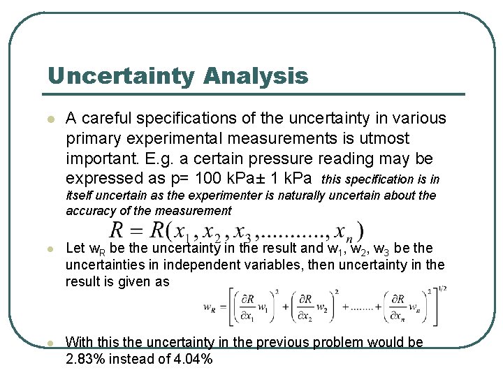
Uncertainty Analysis l A careful specifications of the uncertainty in various primary experimental measurements is utmost important. E. g. a certain pressure reading may be expressed as p= 100 k. Pa± 1 k. Pa this specification is in itself uncertain as the experimenter is naturally uncertain about the accuracy of the measurement l Let w. R be the uncertainty in the result and w 1, w 2, w 3 be the uncertainties in independent variables, then uncertainty in the result is given as l With this the uncertainty in the previous problem would be 2. 83% instead of 4. 04%

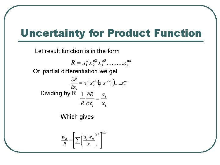
Uncertainty for Product Function Let result function is in the form On partial differentiation we get Dividing by R Which gives

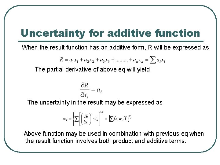
Uncertainty for additive function When the result function has an additive form, R will be expressed as The partial derivative of above eq will yield The uncertainty in the result may be expressed as Above function may be used in combination with previous eq when the result function involves both product and additive terms.

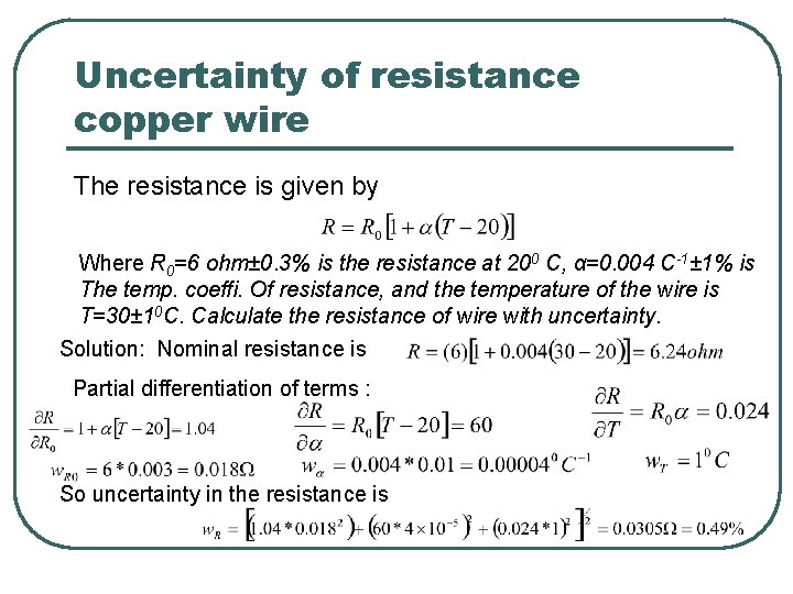
Uncertainty of resistance copper wire The resistance is given by Where R 0=6 ohm± 0. 3% is the resistance at 200 C, α=0. 004 C-1± 1% is The temp. coeffi. Of resistance, and the temperature of the wire is T=30± 10 C. Calculate the resistance of wire with uncertainty. Solution: Nominal resistance is Partial differentiation of terms : So uncertainty in the resistance is

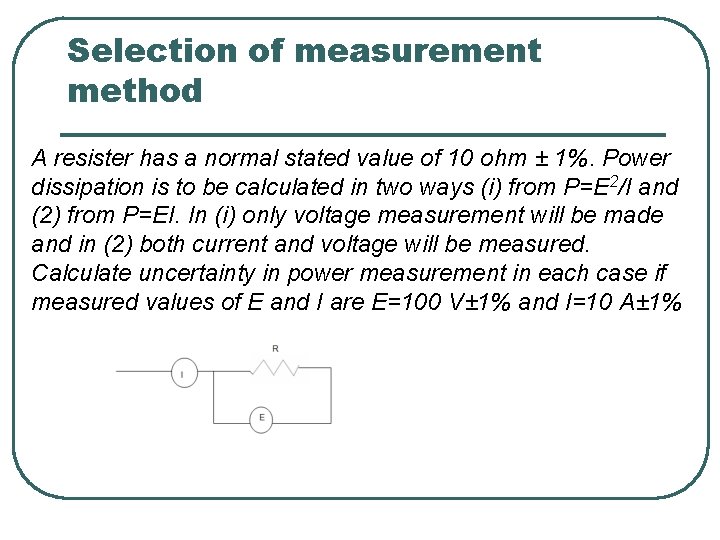
Selection of measurement method A resister has a normal stated value of 10 ohm ± 1%. Power dissipation is to be calculated in two ways (i) from P=E 2/I and (2) from P=EI. In (i) only voltage measurement will be made and in (2) both current and voltage will be measured. Calculate uncertainty in power measurement in each case if measured values of E and I are E=100 V± 1% and I=10 A± 1%

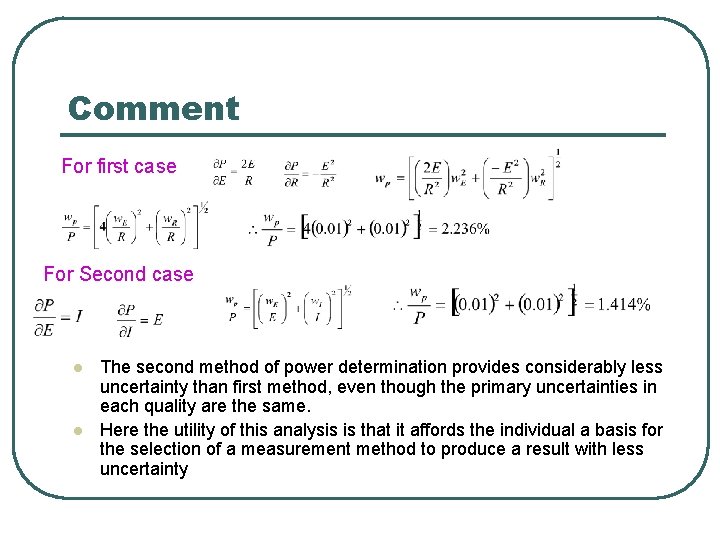
Comment For first case For Second case l l The second method of power determination provides considerably less uncertainty than first method, even though the primary uncertainties in each quality are the same. Here the utility of this analysis is that it affords the individual a basis for the selection of a measurement method to produce a result with less uncertainty

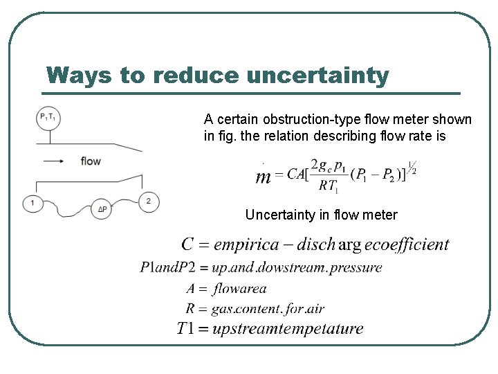
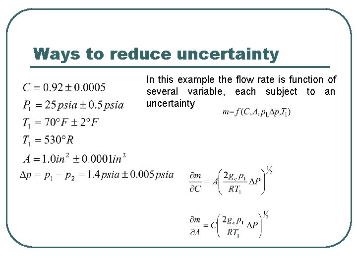
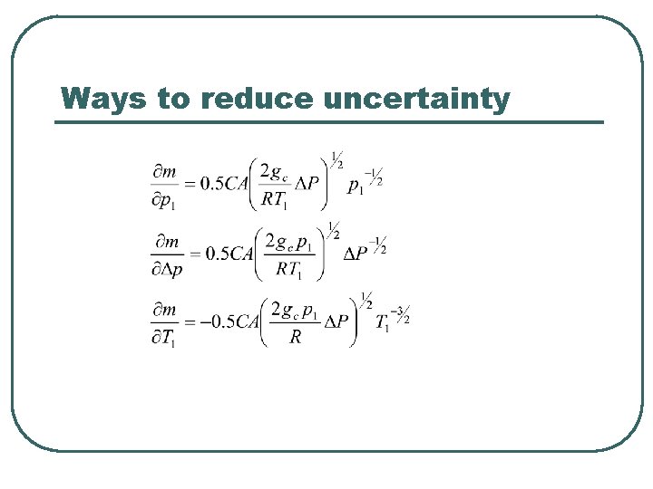
Ways to reduce uncertainty A certain obstruction-type flow meter shown in fig. the relation describing flow rate is Uncertainty in flow meter

Ways to reduce uncertainty In this example the flow rate is function of several variable, each subject to an uncertainty

Ways to reduce uncertainty

Ways to reduce uncertainty

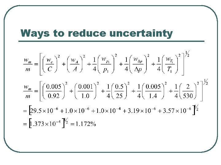
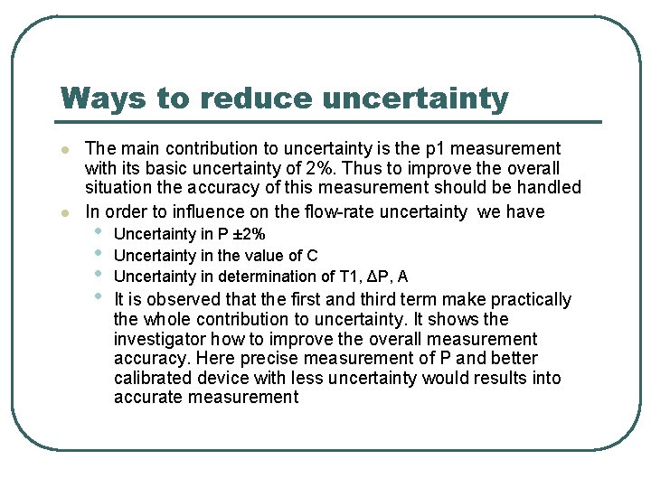
Ways to reduce uncertainty l l The main contribution to uncertainty is the p 1 measurement with its basic uncertainty of 2%. Thus to improve the overall situation the accuracy of this measurement should be handled In order to influence on the flow-rate uncertainty we have • • Uncertainty in P ± 2% Uncertainty in the value of C Uncertainty in determination of T 1, ΔP, A It is observed that the first and third term make practically the whole contribution to uncertainty. It shows the investigator how to improve the overall measurement accuracy. Here precise measurement of P and better calibrated device with less uncertainty would results into accurate measurement

Interpolation Ø To find approx value of function f(x) for an x between difference value of x i. e. x 0, x 1, x 3, ……. . xn at which the value of f(x) are given

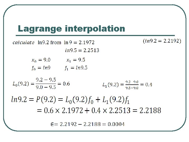
Lagrange interpolation Given (x 0, f 0), (x 1, f 1), (x 2, f 2) Y Y=f(x) error P 1(x) This gives the linear Lagrange polynomial xo x 1 X

Lagrange interpolation

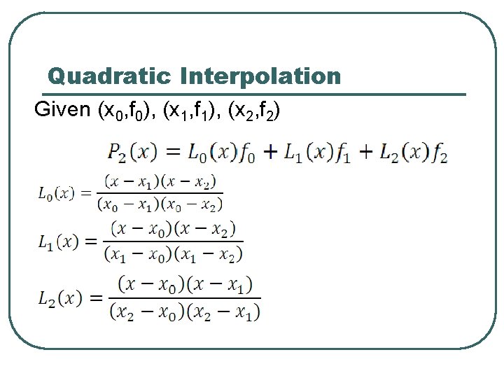
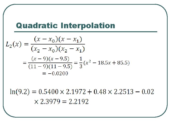
Quadratic Interpolation Given (x 0, f 0), (x 1, f 1), (x 2, f 2)

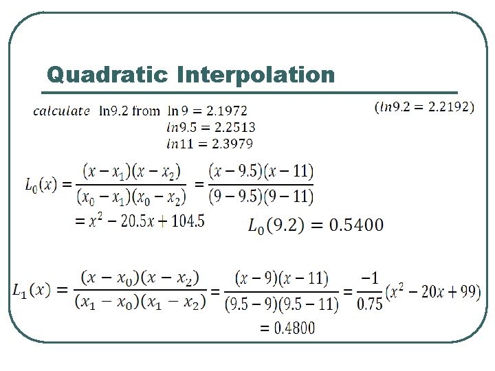
Quadratic Interpolation

Quadratic Interpolation

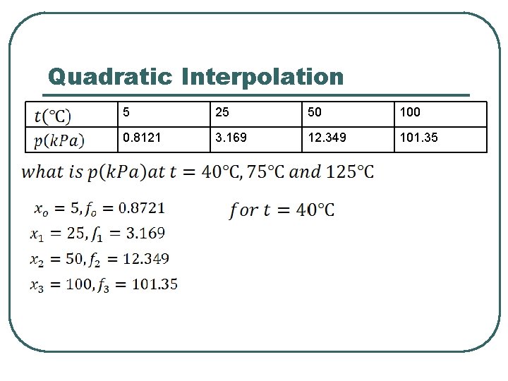
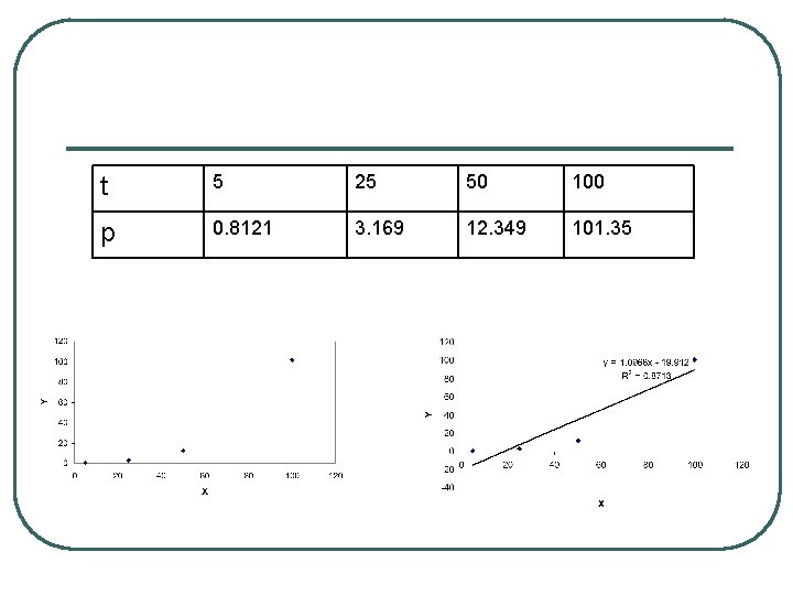
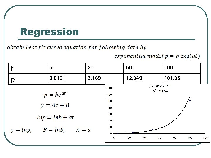
Quadratic Interpolation 5 25 50 100 0. 8121 3. 169 12. 349 101. 35

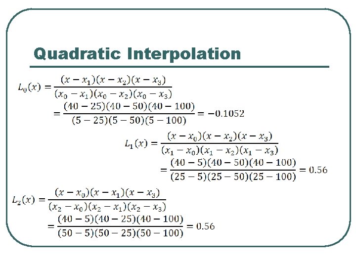
Quadratic Interpolation

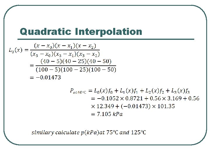
Quadratic Interpolation

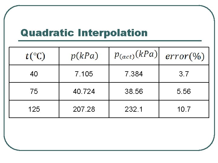
Quadratic Interpolation 40 7. 105 7. 384 3. 7 75 40. 724 38. 56 5. 56 125 207. 28 232. 1 10. 7

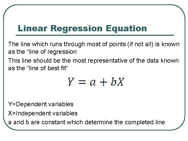
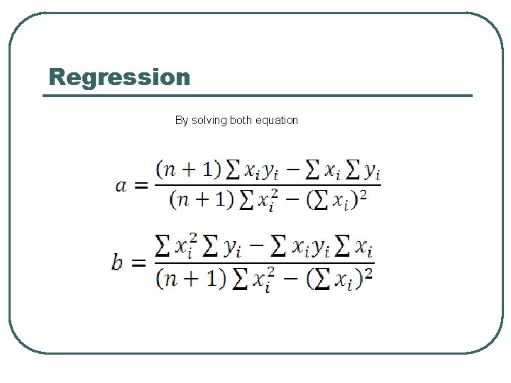
Linear Regression Equation The line which runs through most of points (if not all) is known as the “line of regression This line should be the most representative of the data known as the “line of best fit” Y=Dependent variables X=Independent variables a and b are constant which determine the completed line

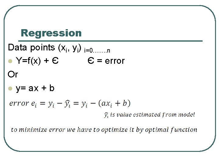
Regression Data points (xi, yi) i=0……. n l Y=f(x) + Є Є = error Or l y= ax + b

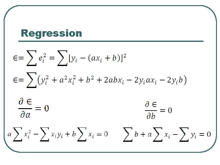
Regression

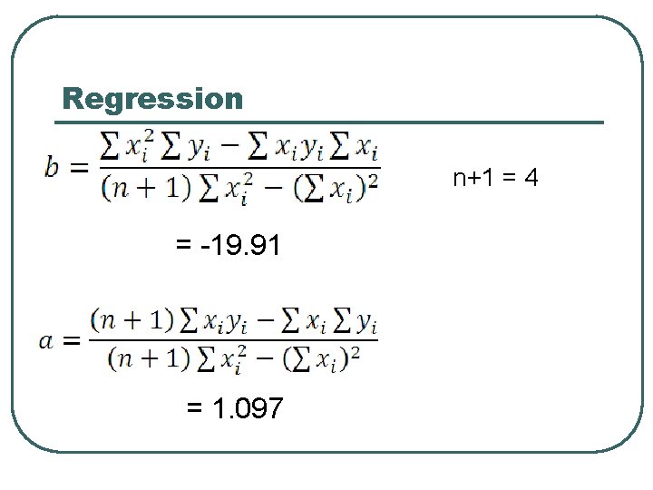
Regression By solving both equation

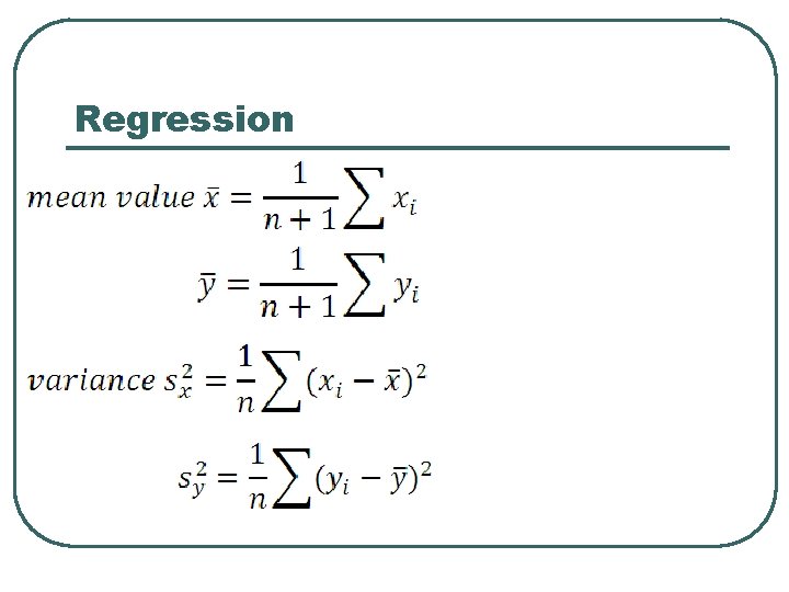
Regression

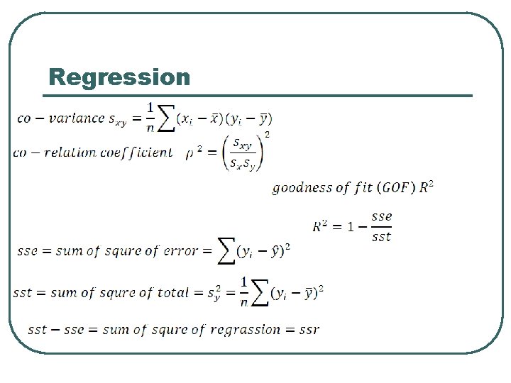
Regression

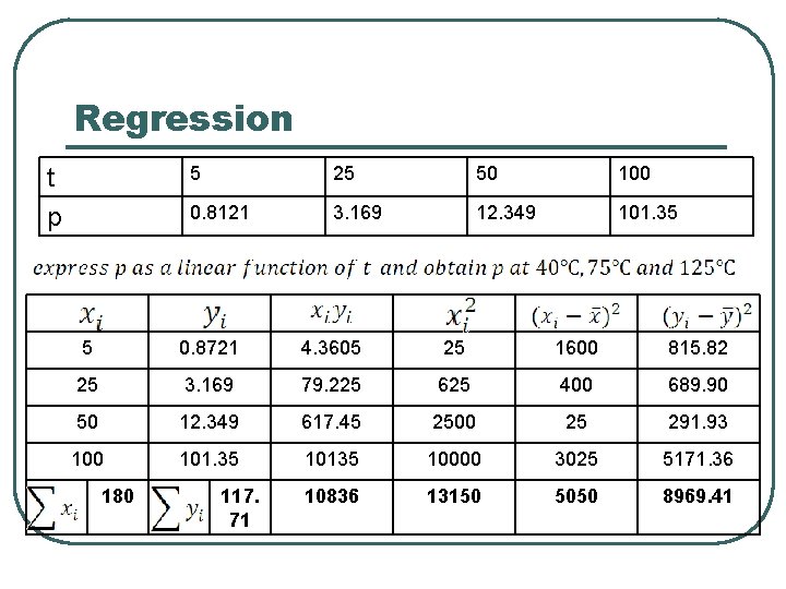
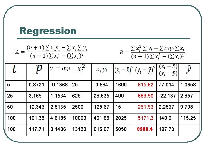
Regression t p 5 25 50 100 0. 8121 3. 169 12. 349 101. 35 5 0. 8721 4. 3605 25 1600 815. 82 25 3. 169 79. 225 625 400 689. 90 50 12. 349 617. 45 2500 25 291. 93 100 101. 35 10135 10000 3025 5171. 36 10836 13150 5050 8969. 41 180 117. 71

t 5 25 50 100 p 0. 8121 3. 169 12. 349 101. 35

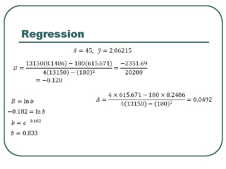
Regression n+1 = 4 = -19. 91 = 1. 097

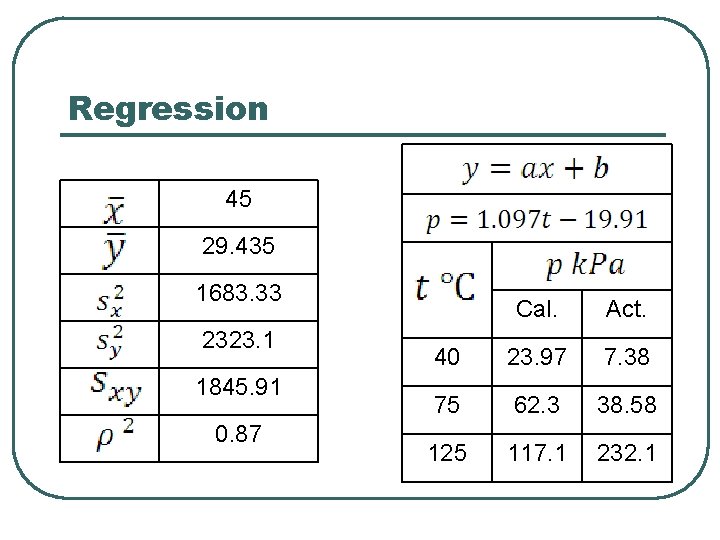
Regression 45 29. 435 1683. 33 2323. 1 1845. 91 0. 87 Cal. Act. 40 23. 97 7. 38 75 62. 3 38. 58 125 117. 1 232. 1

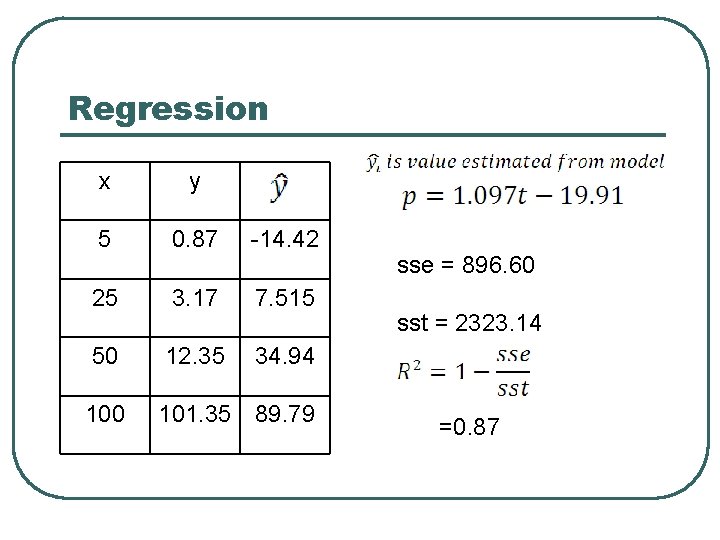
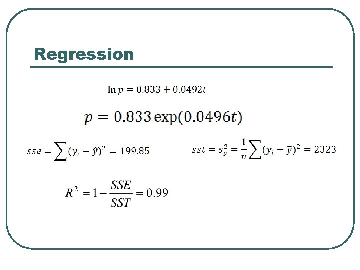
Regression x y 5 0. 87 -14. 42 25 3. 17 7. 515 50 12. 35 34. 94 100 101. 35 89. 79 sse = 896. 60 sst = 2323. 14 =0. 87

Regression t p 5 25 50 100 0. 8121 3. 169 12. 349 101. 35

Regression 5 0. 8721 -0. 1368 25 -0. 684 1600 815. 82 77. 014 25 3. 169 1. 1534 625 28. 835 400 689. 90 -22. 137 2. 857 50 12. 349 2. 5135 2500 125. 67 15 291. 93 2. 2567 9. 798 100 101. 35 4. 6185 10000 461. 85 2025 5171. 3 140. 6 115. 25 180 117. 71 8. 1486 13150 615. 67 5050 8969. 4 197. 73 1. 0658

Regression

Regression

Exponential Model Β>0 Taking log on both sides α Β<0

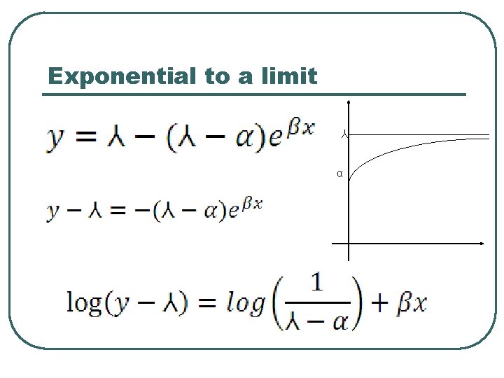
Exponential to a limit Y α

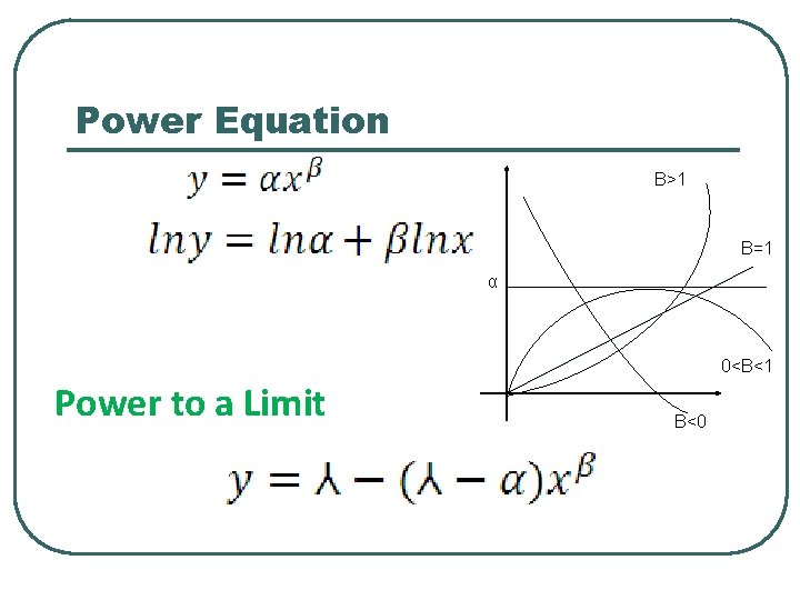
Power Equation Β>1 Β=1 α 0<Β<1 Power to a Limit Β<0

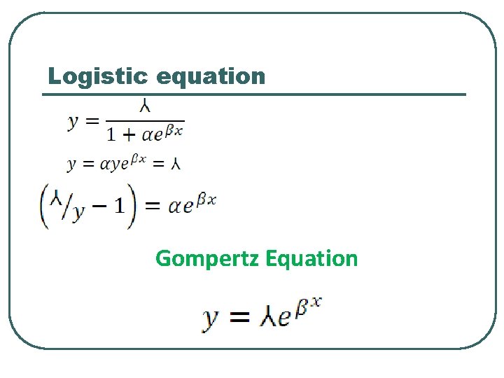
Logistic equation Gompertz Equation

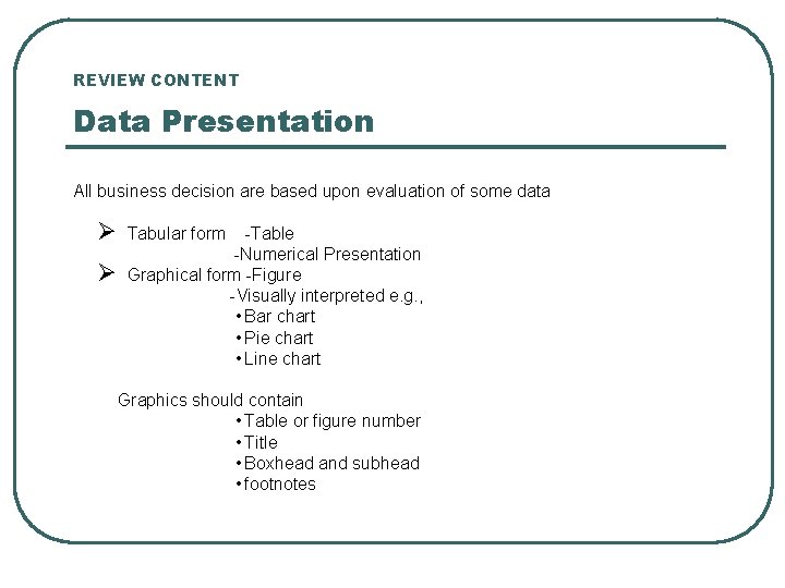
REVIEW CONTENT Data Presentation All business decision are based upon evaluation of some data Ø Ø Tabular form -Table -Numerical Presentation Graphical form -Figure -Visually interpreted e. g. , • Bar chart • Pie chart • Line chart Graphics should contain • Table or figure number • Title • Boxhead and subhead • footnotes

Hypothesis l l Ordinarily hypothesis simply means a mere assumption or some supposition to be proved or disproved. For a researcher- it may be defined as a proposition set forth as an explanation for the occurrence of some specified group of phenomenon accepted as highly probable in the light of established facts. l Research hypothesis is a predictive statement, capable of being tested by scientific methods, that relates an independent variable to some dependent variable.

Characteristics of hypothesis l l l Should be clear and precise Should be capable of being tested Should state relationship between variables Should be limited in scope and be specific Should be stated as far as possible in most simple terms so that same is easily understandable by all concerned Should be consistent with all known facts

Hypothesis Testing Important parametric tests used for testing or hypothesis are: Ø Ø z-test t-test x 2 test F-test Procedure for Testing of Hypothesis Ø Ø Ø State the null hypothesis as well as alternate hypothesis Establish a level of significance (prior to sampling) Choosing a suitable test statistic

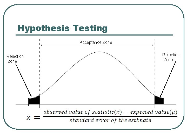
Hypothesis Testing l Rejection Zone Acceptance Zone Rejection Zone

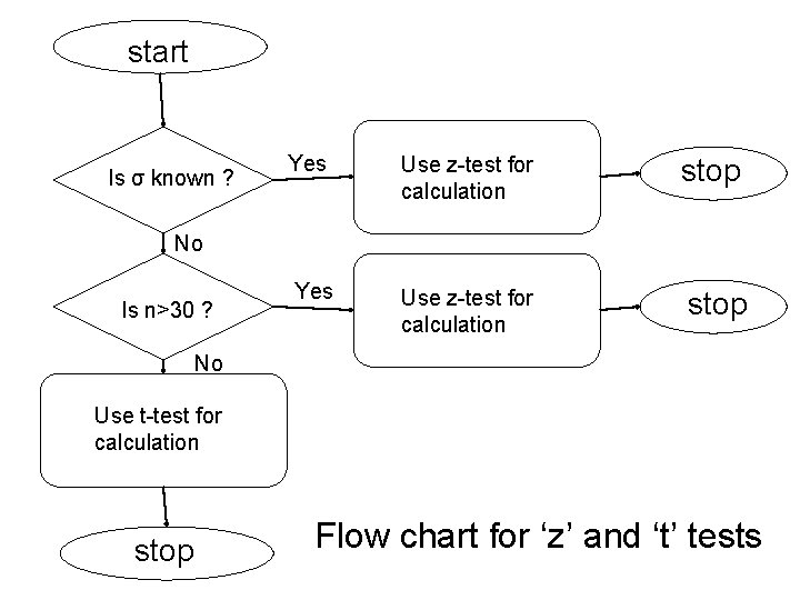
start Is σ known ? Yes Use z-test for calculation stop No Is n>30 ? No Use t-test for calculation stop Flow chart for ‘z’ and ‘t’ tests MTECH THERMAL ENGG 20010 -11

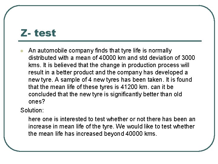
Z- test An automobile company finds that tyre life is normally distributed with a mean of 40000 km and std deviation of 3000 kms. It is believed that the change in production process will result in a better product and the company has developed a new tyre. A sample of 4 new tyres has been taken. It is found that the mean life of these tyres is 41200 km. can it be concluded that the new tyre is significantly better than old ones? Solution: here one is interested to test whether or not there has been an increase in mean life of the tyre. We would like to test whether the mean life has increased beyond 40000 kms. l

l l l Null hypothesis and alternative hypothesis are • • Ho: μ=40000 km H 1: μ≠ 40000 km Significance level is taken as 0. 05 i. e 5 out of every 100 occasions, there is a risk of being wrong in accepting or rejecting the hypothesis The test criterion is z test At 0. 05 level of significance the critical value of z≠ 1. 64 As the computed value of z falls in the rejection region, we reject the Null hypothesis. That is, the alternative hypothesis that life >40000 km is accepted. It is concluded that new tyre is significantly better than old one

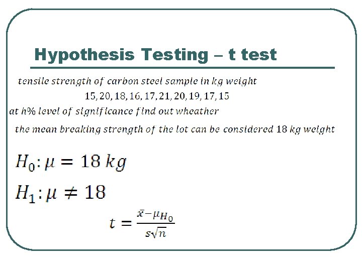
Hypothesis Testing – t test

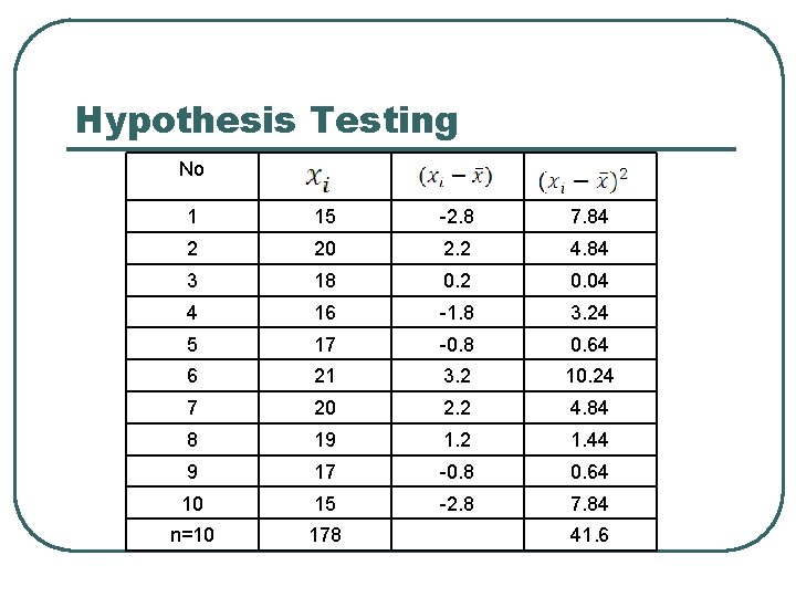
Hypothesis Testing No 1 15 -2. 8 7. 84 2 20 2. 2 4. 84 3 18 0. 2 0. 04 4 16 -1. 8 3. 24 5 17 -0. 8 0. 64 6 21 3. 2 10. 24 7 20 2. 2 4. 84 8 19 1. 2 1. 44 9 17 -0. 8 0. 64 10 15 -2. 8 7. 84 n=10 178 41. 6

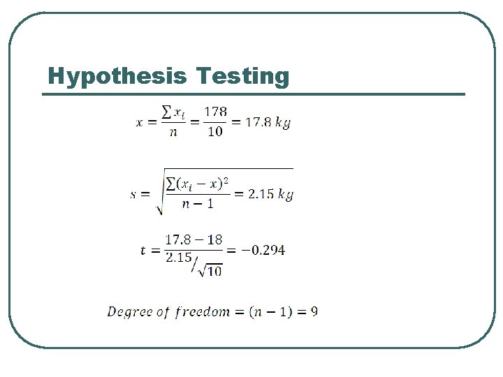
Hypothesis Testing

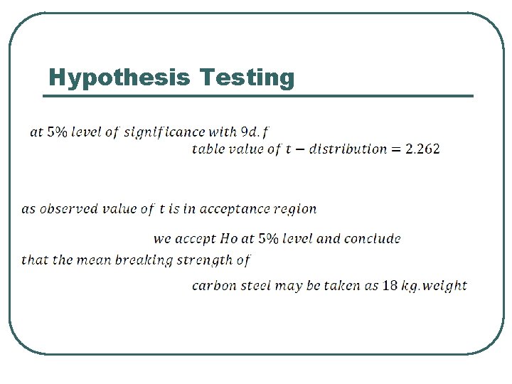
Hypothesis Testing

THANK YOU

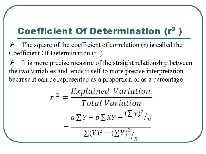
Coefficient Of Determination (r 2 ) Ø The square of the coefficient of correlation (r) is called the Coefficient Of Determination (r 2 ) Ø It is more precise measure of the straight relationship between the two variables and lends it self to more precise interpretation because it can be represented as a proportion or as a percentage

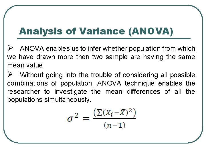
Analysis of Variance (ANOVA) Ø ANOVA enables us to infer whether population from which we have drawn more then two sample are having the same mean value Ø Without going into the trouble of considering all possible combinations of population, ANOVA technique enables the researcher to investigate the mean differences of all the populations simultaneously.