730 Lecture 20 Todays lecture 322021 730 lecture

730 Lecture 20 Today’s lecture: 3/2/2021 730 lecture 20 1

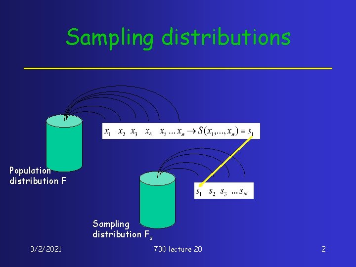
Sampling distributions Population distribution F Sampling distribution Fs 3/2/2021 730 lecture 20 2

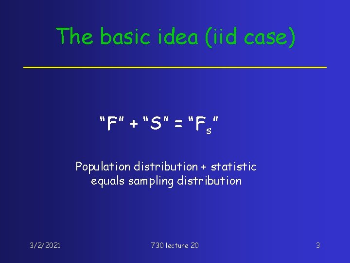
The basic idea (iid case) “F” + “S” = “Fs” Population distribution + statistic equals sampling distribution 3/2/2021 730 lecture 20 3

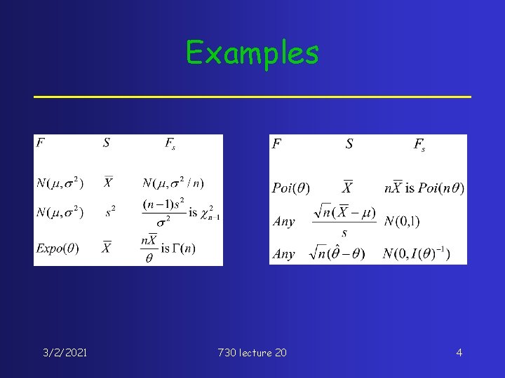
Examples 3/2/2021 730 lecture 20 4

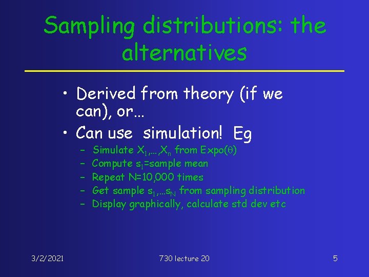
Sampling distributions: the alternatives • Derived from theory (if we can), or… • Can use simulation! Eg – – – 3/2/2021 Simulate X 1, …, Xn from Expo(q) Compute s 1=sample mean Repeat N=10, 000 times Get sample s 1, …s. N from sampling distribution Display graphically, calculate std dev etc 730 lecture 20 5

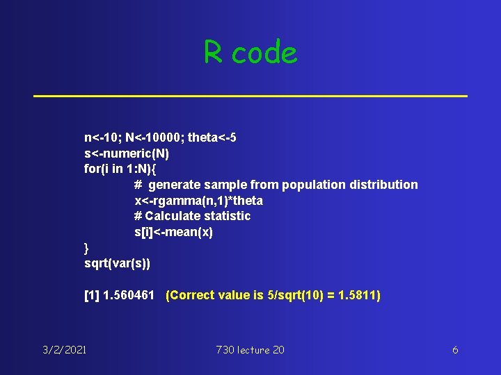
R code n<-10; N<-10000; theta<-5 s<-numeric(N) for(i in 1: N){ # generate sample from population distribution x<-rgamma(n, 1)*theta # Calculate statistic s[i]<-mean(x) } sqrt(var(s)) [1] 1. 560461 (Correct value is 5/sqrt(10) = 1. 5811) 3/2/2021 730 lecture 20 6

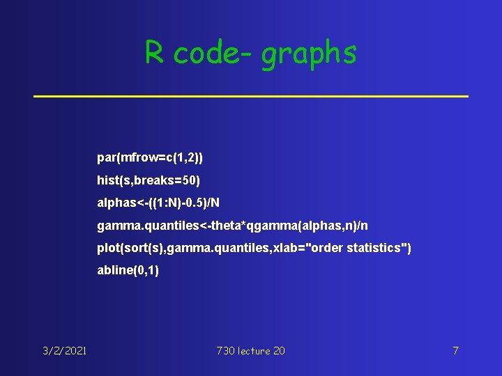
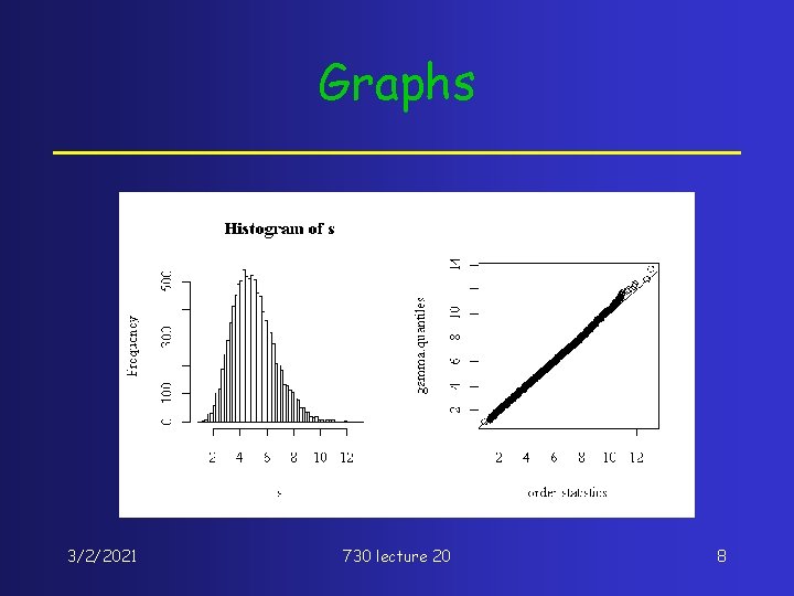
R code- graphs par(mfrow=c(1, 2)) hist(s, breaks=50) alphas<-((1: N)-0. 5)/N gamma. quantiles<-theta*qgamma(alphas, n)/n plot(sort(s), gamma. quantiles, xlab="order statistics") abline(0, 1) 3/2/2021 730 lecture 20 7

Graphs 3/2/2021 730 lecture 20 8

The big problem…. • • 3/2/2021 In practice we don’t know F! What can we do? Estimate F! How? 730 lecture 20 9

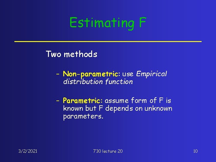
Estimating F Two methods – Non-parametric: use Empirical distribution function – Parametric: assume form of F is known but F depends on unknown parameters. 3/2/2021 730 lecture 20 10

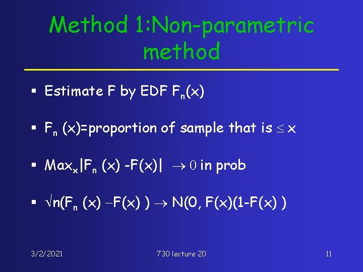
Method 1: Non-parametric method § Estimate F by EDF Fn(x) § Fn (x)=proportion of sample that is £ x § Maxx|Fn (x) -F(x)| ® 0 in prob § Ön(Fn (x) -F(x) ) ® N(0, F(x)(1 -F(x) ) 3/2/2021 730 lecture 20 11

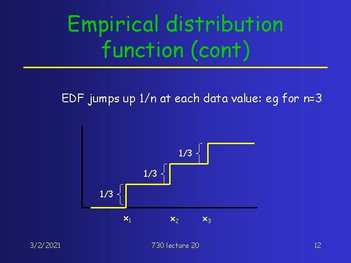
Empirical distribution function (cont) EDF jumps up 1/n at each data value: eg for n=3 1/3 1/3 x 1 3/2/2021 x 2 730 lecture 20 x 3 12

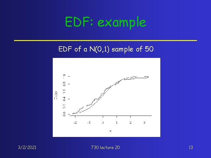
EDF: example EDF of a N(0, 1) sample of 50 3/2/2021 730 lecture 20 13

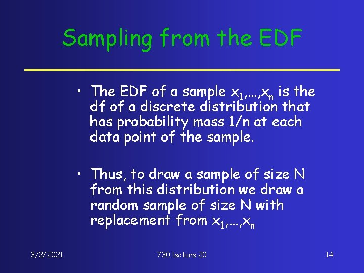
Sampling from the EDF • The EDF of a sample x 1, …, xn is the df of a discrete distribution that has probability mass 1/n at each data point of the sample. • Thus, to draw a sample of size N from this distribution we draw a random sample of size N with replacement from x 1, …, xn 3/2/2021 730 lecture 20 14

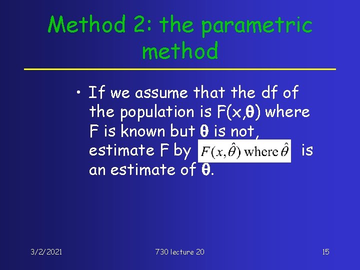
Method 2: the parametric method • If we assume that the df of the population is F(x, q) where F is known but q is not, estimate F by is an estimate of q. 3/2/2021 730 lecture 20 15

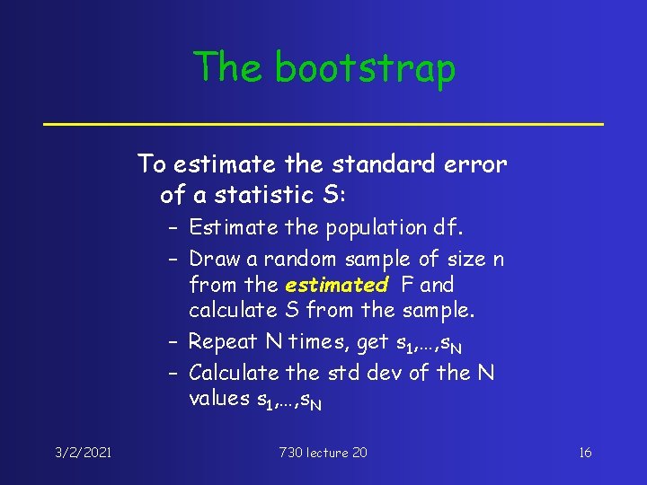
The bootstrap To estimate the standard error of a statistic S: – Estimate the population df. – Draw a random sample of size n from the estimated F and calculate S from the sample. – Repeat N times, get s 1, …, s. N – Calculate the std dev of the N values s 1, …, s. N 3/2/2021 730 lecture 20 16

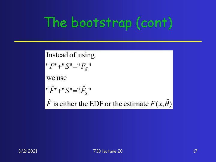
The bootstrap (cont) 3/2/2021 730 lecture 20 17

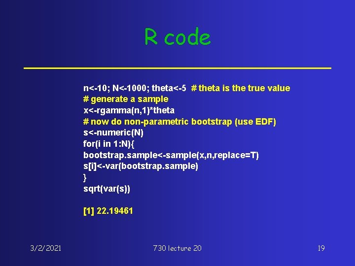
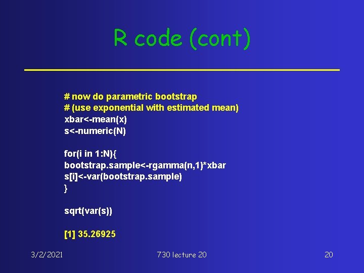
Example • Suppose we want to estimate the standard error of the sample variance. The population distribution is exponential and n=10. 3/2/2021 730 lecture 20 18

R code n<-10; N<-1000; theta<-5 # theta is the true value # generate a sample x<-rgamma(n, 1)*theta # now do non-parametric bootstrap (use EDF) s<-numeric(N) for(i in 1: N){ bootstrap. sample<-sample(x, n, replace=T) s[i]<-var(bootstrap. sample) } sqrt(var(s)) [1] 22. 19461 3/2/2021 730 lecture 20 19

R code (cont) # now do parametric bootstrap # (use exponential with estimated mean) xbar<-mean(x) s<-numeric(N) for(i in 1: N){ bootstrap. sample<-rgamma(n, 1)*xbar s[i]<-var(bootstrap. sample) } sqrt(var(s)) [1] 35. 26925 3/2/2021 730 lecture 20 20

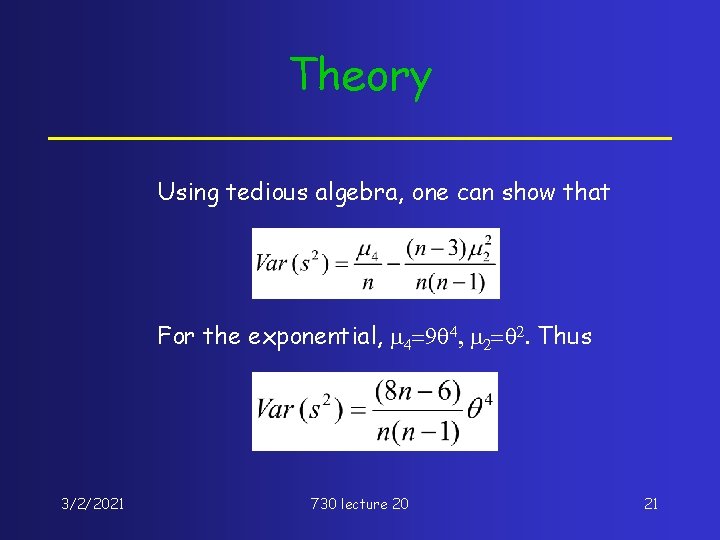
Theory Using tedious algebra, one can show that For the exponential, m 4=9 q 4, m 2=q 2. Thus 3/2/2021 730 lecture 20 21

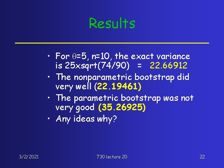
Results • For q=5, n=10, the exact variance is 25 xsqrt(74/90) = 22. 66912 • The nonparametric bootstrap did very well (22. 19461) • The parametric bootstrap was not very good (35. 26925) • Any ideas why? 3/2/2021 730 lecture 20 22