10 Quantum Monte Carlo Methods Variational Principle For

10. Quantum Monte Carlo Methods

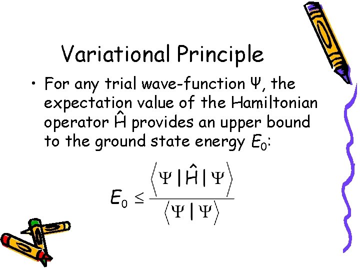
Variational Principle • For any trial wave-function Ψ, the expectation value of the Hamiltonian operator Ĥ provides an upper bound to the ground state energy E 0:

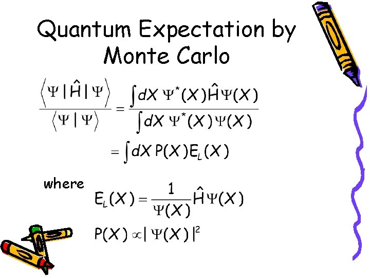
Quantum Expectation by Monte Carlo where

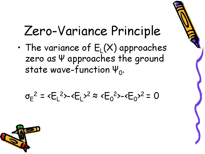
Zero-Variance Principle • The variance of EL(X) approaches zero as Ψ approaches the ground state wave-function Ψ 0. σE 2 = <EL 2>-<EL>2 ≈ <E 02>-<E 0>2 = 0

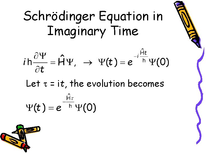
Schrödinger Equation in Imaginary Time Let = it, the evolution becomes

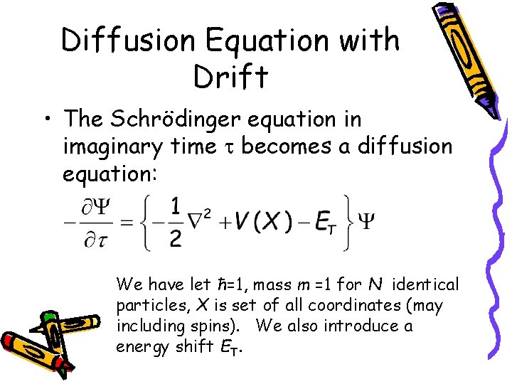
Diffusion Equation with Drift • The Schrödinger equation in imaginary time becomes a diffusion equation: We have let ħ=1, mass m =1 for N identical particles, X is set of all coordinates (may including spins). We also introduce a energy shift ET.

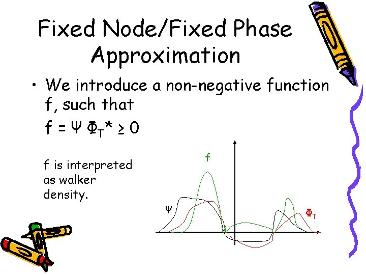
Fixed Node/Fixed Phase Approximation • We introduce a non-negative function f, such that f = Ψ ΦT * ≥ 0 f is interpreted as walker density. f Ψ ΦT

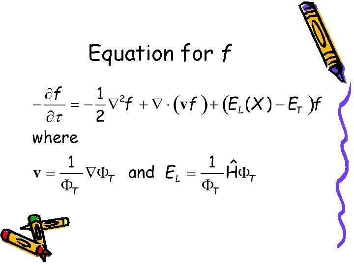
Equation for f

Monte Carlo Simulation of the Diffusion Equation • If we have only the first term -½ 2 f, it is a pure random walk. • If we have first and second term, it describes a diffusion with drift velocity v. • The last term represents birth-death of the walkers.

Walker Space X The population of the walkers is proportional to the solution f(X).

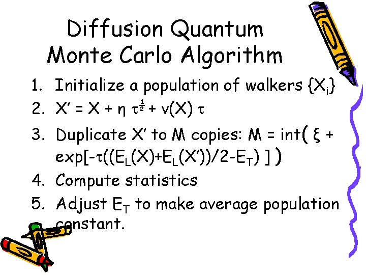
Diffusion Quantum Monte Carlo Algorithm 1. Initialize a population of walkers {Xi} 2. X’ = X + η ½ + v(X) 3. Duplicate X’ to M copies: M = int( ξ + exp[- ((EL(X)+EL(X’))/2 -ET) ] ) 4. Compute statistics 5. Adjust ET to make average population constant.

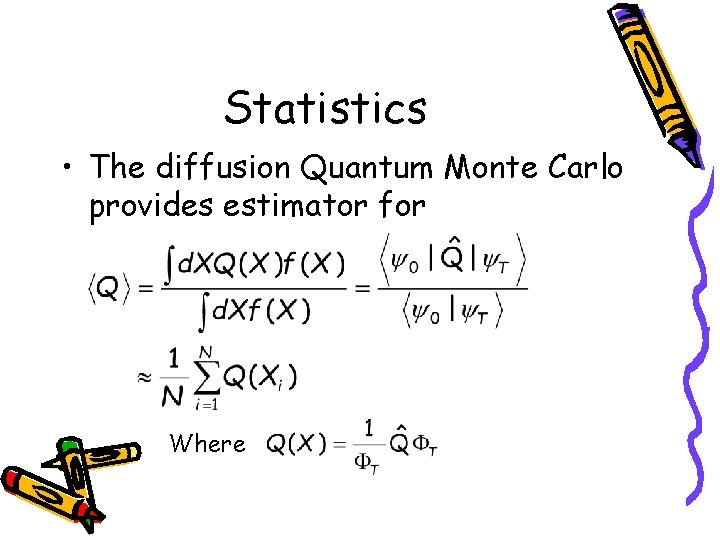
Statistics • The diffusion Quantum Monte Carlo provides estimator for Where

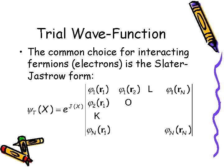
Trial Wave-Function • The common choice for interacting fermions (electrons) is the Slater. Jastrow form:

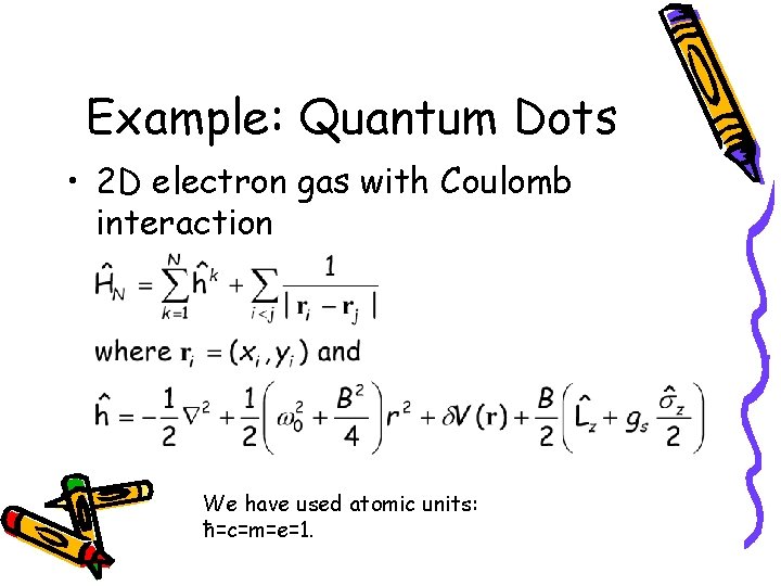
Example: Quantum Dots • 2 D electron gas with Coulomb interaction We have used atomic units: ħ=c=m=e=1.

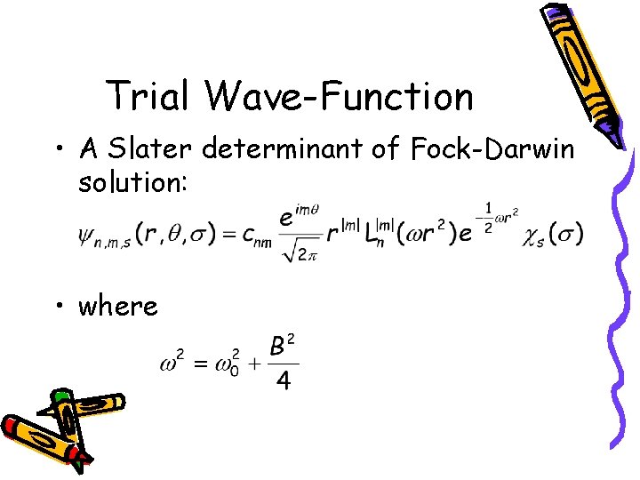
Trial Wave-Function • A Slater determinant of Fock-Darwin solution: • where

Six-Electron Groundstate Energy The (L, S) values are the total orbital angular momentum L and total Pauli spin S. From J S Wang, A D Güçlü and H Guo, unpublished

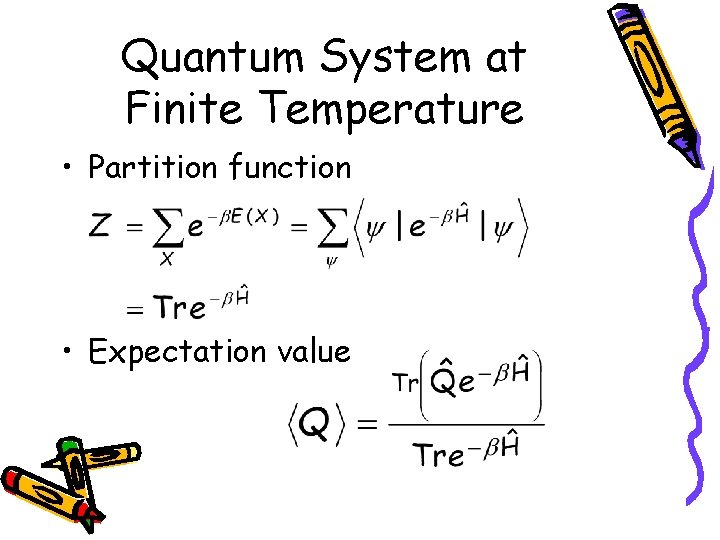
Quantum System at Finite Temperature • Partition function • Expectation value

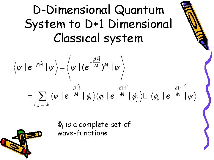
D-Dimensional Quantum System to D+1 Dimensional Classical system Φi is a complete set of wave-functions

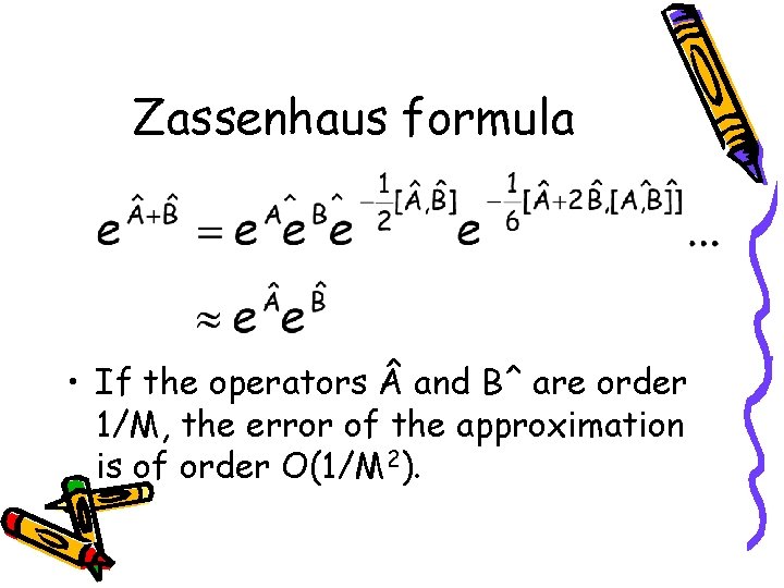
Zassenhaus formula • If the operators and Bˆ are order 1/M, the error of the approximation is of order O(1/M 2).

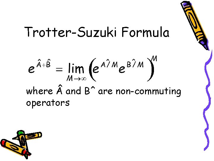
Trotter-Suzuki Formula where and Bˆ are non-commuting operators

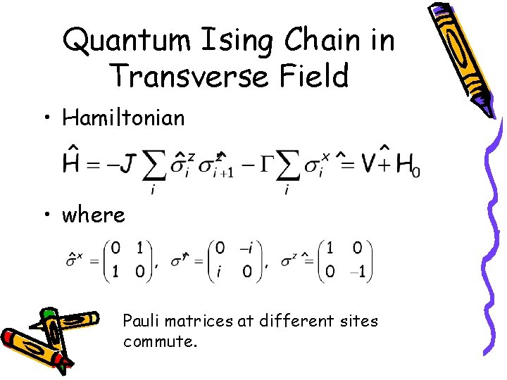
Quantum Ising Chain in Transverse Field • Hamiltonian • where Pauli matrices at different sites commute.

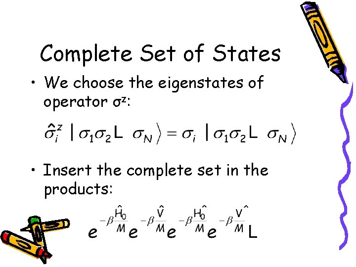
Complete Set of States • We choose the eigenstates of operator σz: • Insert the complete set in the products:

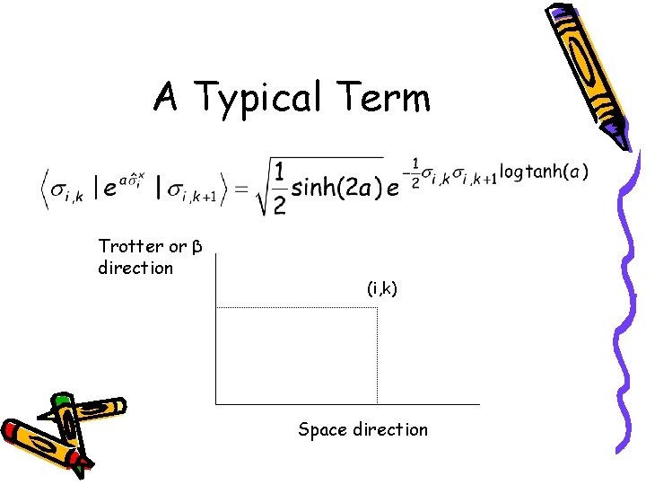
A Typical Term Trotter or β direction (i, k) Space direction

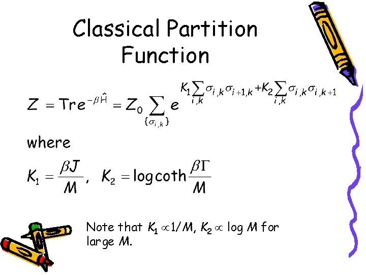
Classical Partition Function Note that K 1 1/M, K 2 log M for large M.

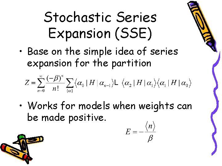
Stochastic Series Expansion (SSE) • Base on the simple idea of series expansion for the partition • Works for models when weights can be made positive.

Spin ½ Heisenberg Model, “World Lines” Hb = I + H 1 + H 2, open bar indicates diagonal part of the Hamiltonian H 1, solid bar off-diagonal Hamiltonian H 2, flipping the spins. Red dot - spin up, open dot - down spin. “time” or “space”