Wind loading and structural response Lecture 13 Dr

Wind loading and structural response Lecture 13 Dr. J. D. Holmes Effective static loading distributions

Effective static loading distributions • Static load distributions which give correct peak load effects under fluctuating wind loading Separately calculate e. s. l. d s for : • mean component • background component • resonant components • Generally e. s. l. d. s depend on load effect (e. g. bending moment, shear)

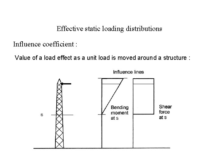
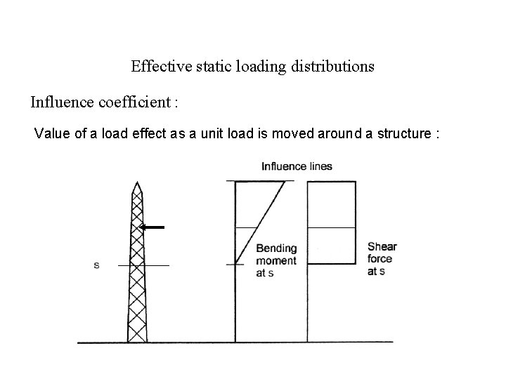
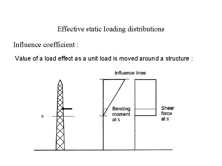
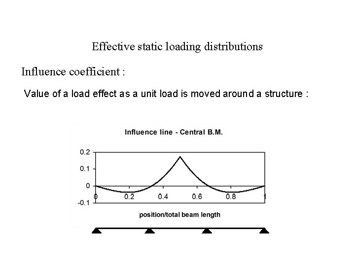
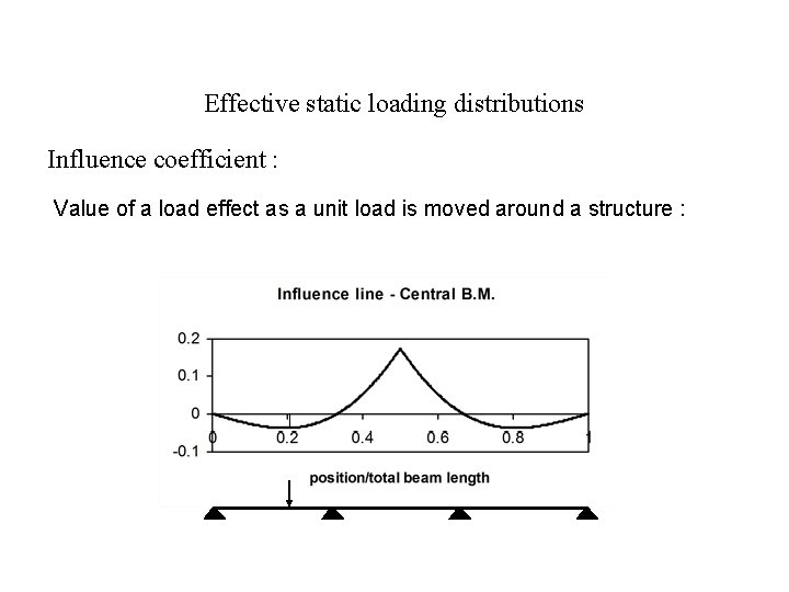
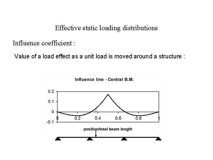
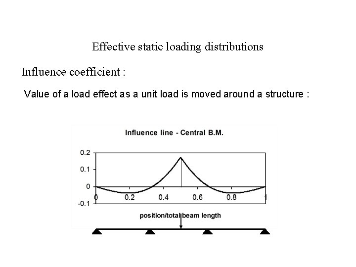
Effective static loading distributions Influence coefficient : Value of a load effect as a unit load is moved around a structure :

Effective static loading distributions Influence coefficient : Value of a load effect as a unit load is moved around a structure :

Effective static loading distributions Influence coefficient : Value of a load effect as a unit load is moved around a structure :

Effective static loading distributions Influence coefficient : Value of a load effect as a unit load is moved around a structure :

Effective static loading distributions Influence coefficient : Value of a load effect as a unit load is moved around a structure :

Effective static loading distributions Influence coefficient : Value of a load effect as a unit load is moved around a structure :

Effective static loading distributions Influence coefficient : Value of a load effect as a unit load is moved around a structure :

Effective static loading distributions Influence coefficient : Value of a load effect as a unit load is moved around a structure :

Effective static loading distributions Influence coefficient : Value of a load effect as a unit load is moved around a structure :

Effective static loading distributions Influence coefficient : Value of a load effect as a unit load is moved around a structure :

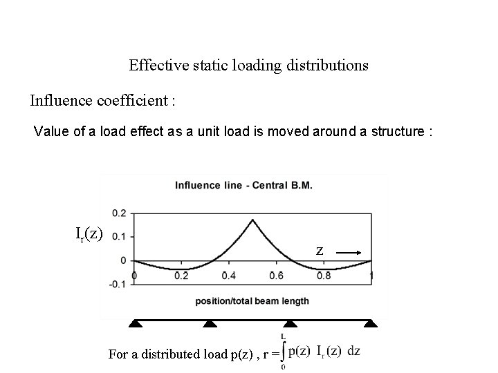
Effective static loading distributions Influence coefficient : Value of a load effect as a unit load is moved around a structure : Ir(z) z For a distributed load p(z) , r =

Effective static loading distributions Mean component p(z) = [0. 5 a Uh 2] Cp on a tower : f (z) = [0. 5 a U(z)2] Cd b(z) (per unit height)

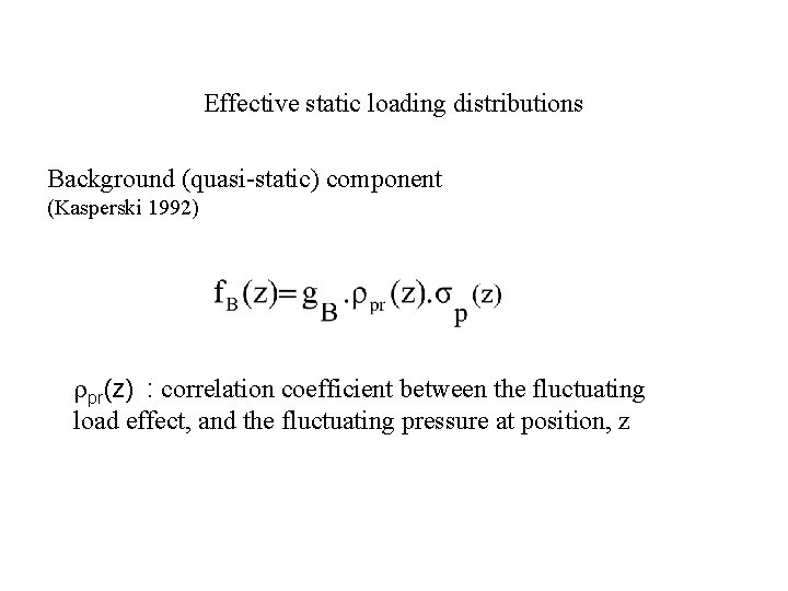
Effective static loading distributions Background (quasi-static) component (Kasperski 1992) pr(z) : correlation coefficient between the fluctuating load effect, and the fluctuating pressure at position, z

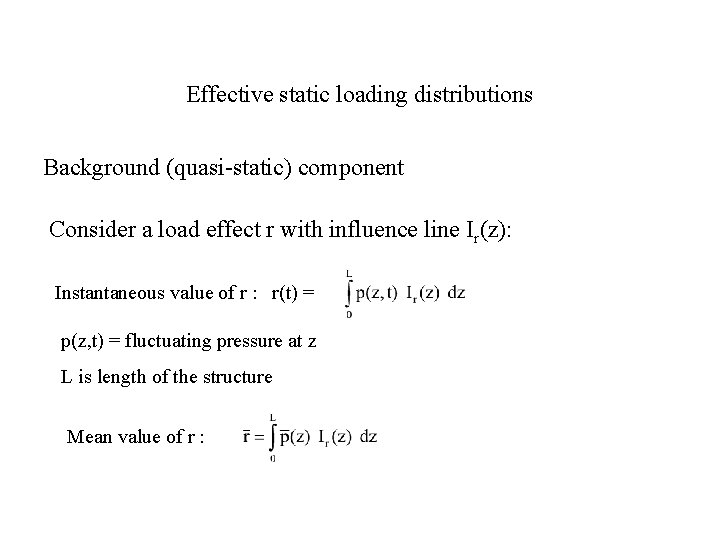
Effective static loading distributions Background (quasi-static) component Consider a load effect r with influence line Ir(z): Instantaneous value of r : r(t) = p(z, t) = fluctuating pressure at z L is length of the structure Mean value of r :

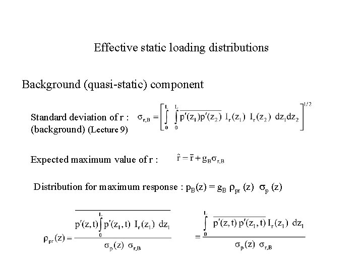
Effective static loading distributions Background (quasi-static) component Standard deviation of r : (background) (Lecture 9) Expected maximum value of r : Distribution for maximum response : p. B(z) = g. B pr (z) p (z)

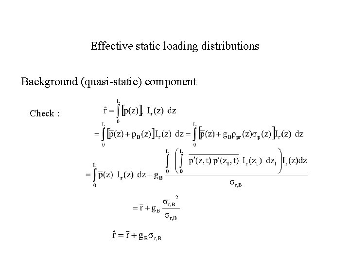
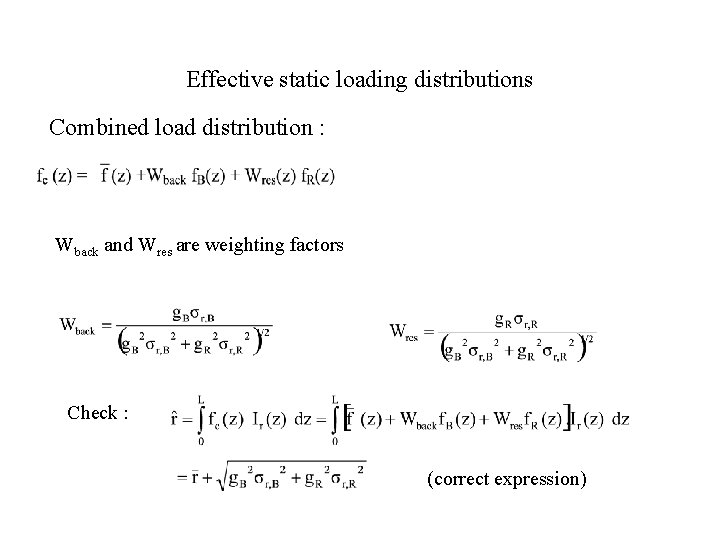
Effective static loading distributions Background (quasi-static) component Check :

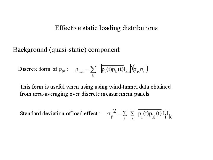
Effective static loading distributions Background (quasi-static) component Discrete form of pr : This form is useful when using wind-tunnel data obtained from area-averaging over discrete measurement panels Standard deviation of load effect :

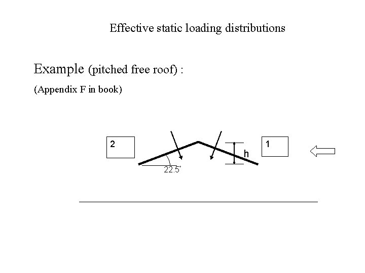
Effective static loading distributions Example (pitched free roof) : (Appendix F in book) 2 h 22. 5 1

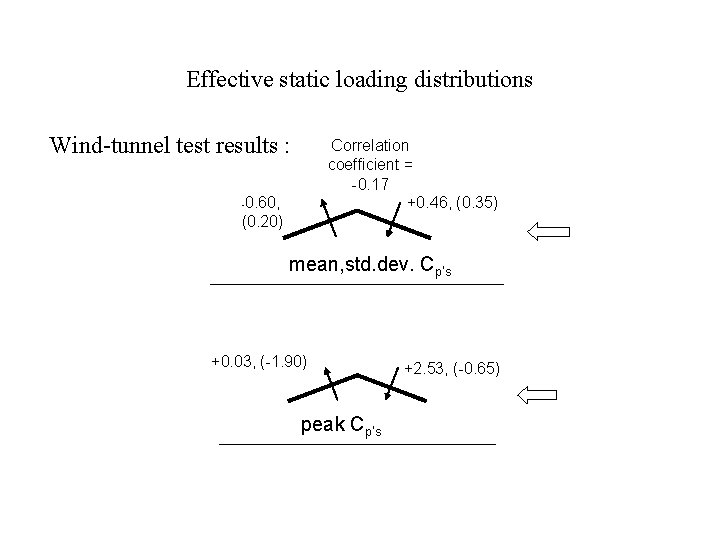
Effective static loading distributions Wind-tunnel test results : Correlation coefficient = -0. 17 +0. 46, (0. 35) 0. 60, (0. 20) - mean, std. dev. Cp’s +0. 03, (-1. 90) peak Cp’s +2. 53, (-0. 65)

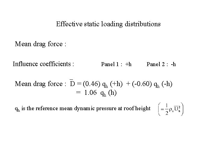
Effective static loading distributions Mean drag force : Influence coefficients : Panel 1 : +h Panel 2 : -h Mean drag force : D = (0. 46) qh (+h) + (-0. 60) qh (-h) = 1. 06 qh (h) qh is the reference mean dynamic pressure at roof height

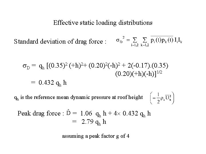
Effective static loading distributions Standard deviation of drag force : D = qh [(0. 35)2 (+h)2+ (0. 20)2(-h)2 + 2(-0. 17). (0. 35) (0. 20)(+h)(-h)]1/2 = 0. 432 qh h qh is the reference mean dynamic pressure at roof height Peak drag force : = 1. 06 qh h + 4 0. 432 qh h = 2. 79 qh h assuming a peak factor g of 4

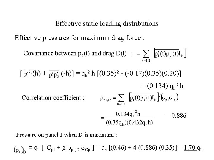
Effective static loading distributions Effective pressures for maximum drag force : Covariance between p 1(t) and drag D(t) : [ . (h) + (-h)] = qh 2 h [(0. 35)2 - (-0. 17)(0. 35)(0. 20)] = (0. 134) qh 2 h Correlation coefficient : = 0. 886 Pressure on panel 1 when D is maximum : = qh [ Cp 1 + g p 1, D Cp 1] = qh [(0. 46) + 4 (0. 886) (0. 35)] = 1. 70 qh

Effective static loading distributions Effective pressures for maximum drag force : Covariance between p 2(t) and drag D(t) : [ . (h) + (-h)] = qh 2 h [ (-0. 17)(0. 20)(0. 35)- (0. 20)2 )] = -(0. 052) qh 2 h Correlation coefficient : = -0. 602 Pressure on panel 2 when D is maximum : = qh [ Cp 2 + g p 2, D Cp 2] = qh [(-0. 60) + 4 (-0. 602) (0. 20)] = -1. 08 qh

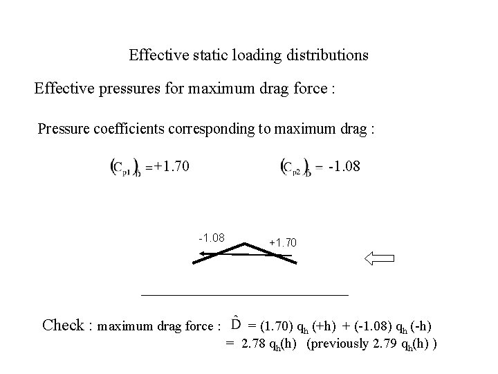
Effective static loading distributions Effective pressures for maximum drag force : Pressure coefficients corresponding to maximum drag : -1. 08 +1. 70 -1. 08 Check : maximum drag force : +1. 70 = (1. 70) qh (+h) + (-1. 08) qh (-h) = 2. 78 qh(h) (previously 2. 79 qh(h) )

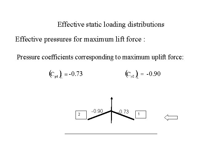
Effective static loading distributions Effective pressures for maximum lift force : Pressure coefficients corresponding to maximum uplift force: -0. 90 -0. 73 2 -0. 90 -0. 73 1

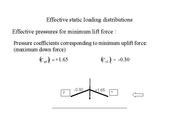
Effective static loading distributions Effective pressures for minimum lift force : Pressure coefficients corresponding to minimum uplift force: (maximum down force) -0. 30 +1. 65 2 -0. 30 +1. 65 1

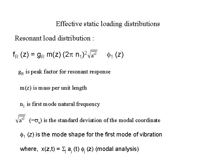
Effective static loading distributions Resonant load distribution : f. R (z) = g. R m(z) (2 n 1)2 1 (z) g. R is peak factor for resonant response m(z) is mass per unit length n 1 is first mode natural frequency (= a) is the standard deviation of the modal coordinate 1 (z) is the mode shape for the first mode of vibration where, x(z, t) = j aj (t) j (z) (modal analysis)

Effective static loading distributions Combined load distribution : Wback and Wres are weighting factors Check : (correct expression)

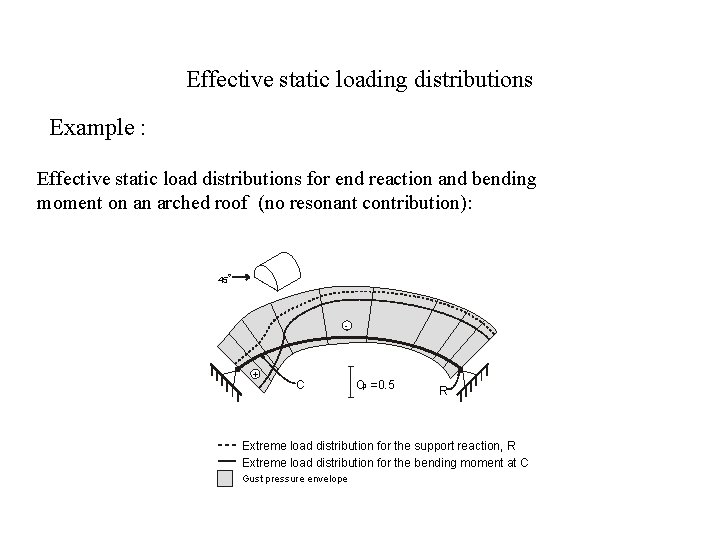
Effective static loading distributions Example : Effective static load distributions for end reaction and bending moment on an arched roof (no resonant contribution): 45 - + C Cp =0. 5 R Extreme load distribution for the support reaction, R Extreme load distribution for the bending moment at C Gust pressure envelope

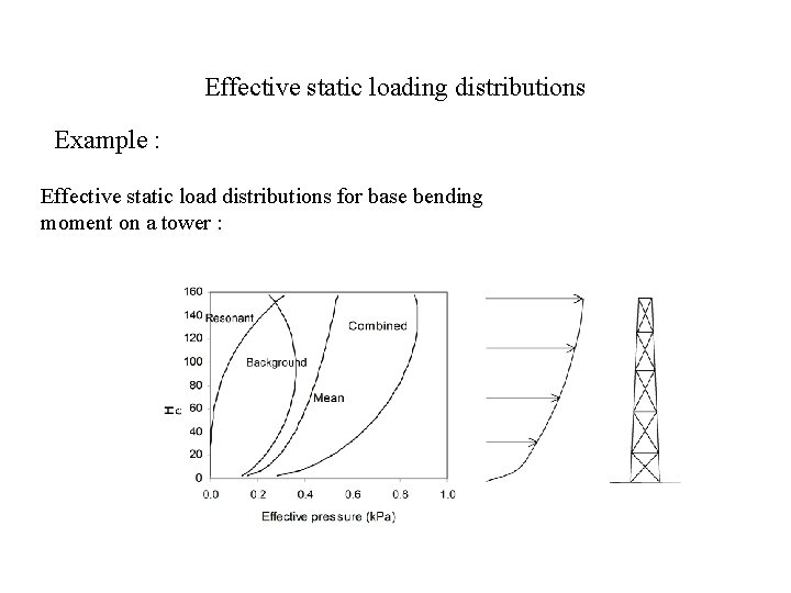
Effective static loading distributions Example : Effective static load distributions for base bending moment on a tower :

End of Lecture 13 John Holmes 225 -405 -3789 JHolmes@lsu. edu