Wind loading and structural response Lecture 4 Dr

Wind loading and structural response Lecture 4 Dr. J. D. Holmes Prediction of design wind speeds

Prediction of design wind speeds • Historical : 1928. Fisher and Tippett. Three asymptotic extreme value distributions 1954. Gumbel method of fitting extremes. Still widely used for windspeeds. 1955. Jenkinson. Generalized extreme value distribution 1977. Gomes and Vickery. Separation of storm types 1982. Simiu. First comprehensive analysis of U. S. historical extreme wind speeds. Sampling errors. 1990. Davison and Smith. Excesses over threshold method. 1998. Peterka and Shahid. Re-analysis of U. S. data - ‘superstations’

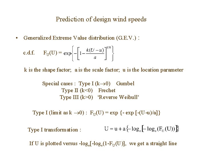
Prediction of design wind speeds • Generalized Extreme Value distribution (G. E. V. ) : c. d. f. FU(U) = k is the shape factor; a is the scale factor; u is the location parameter Special cases : Type I (k 0) Gumbel Type II (k<0) Frechet Type III (k>0) ‘Reverse Weibull’ Type I (limit as k 0) : FU(U) = exp {- exp [-(U-u)/a]} Type I transformation : If U is plotted versus -loge[-loge(1 -FU(U)], we get a straight line

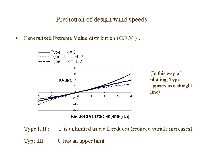
Prediction of design wind speeds • Generalized Extreme Value distribution (G. E. V. ) : Type I k = 0 Type III k = +0. 2 Type II k = -0. 2 8 (In this way of plotting, Type I appears as a straight line) 6 (U-u)/a 4 2 0 -3 -2 -1 -2 0 1 2 3 4 -4 -6 Reduced variate : -ln[-ln(FU(U)] Type I, II : U is unlimited as c. d. f. reduces (reduced variate increases) Type III: U has an upper limit

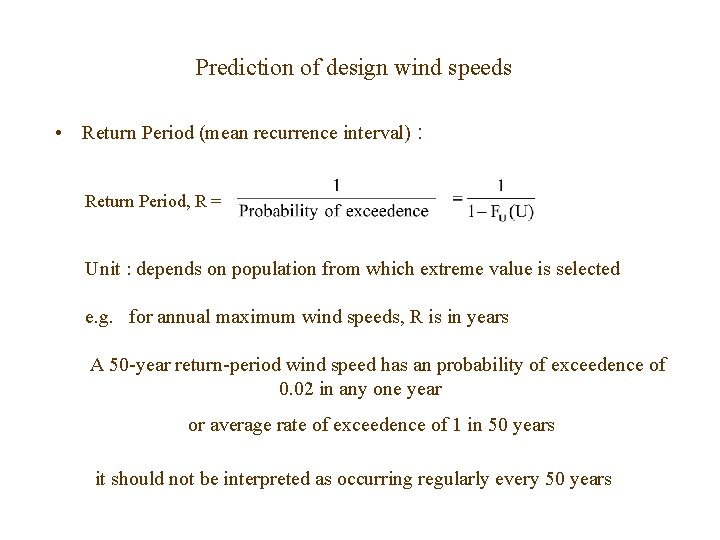
Prediction of design wind speeds • Return Period (mean recurrence interval) : Return Period, R = Unit : depends on population from which extreme value is selected e. g. for annual maximum wind speeds, R is in years A 50 -year return-period wind speed has an probability of exceedence of 0. 02 in any one year or average rate of exceedence of 1 in 50 years it should not be interpreted as occurring regularly every 50 years

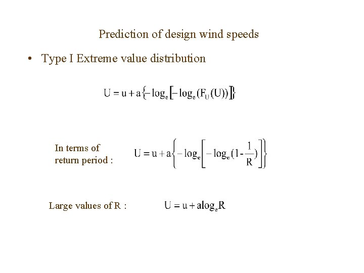
Prediction of design wind speeds • Type I Extreme value distribution In terms of return period : Large values of R :

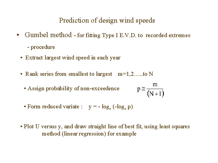
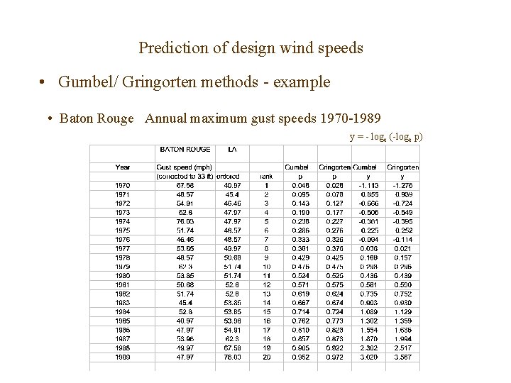
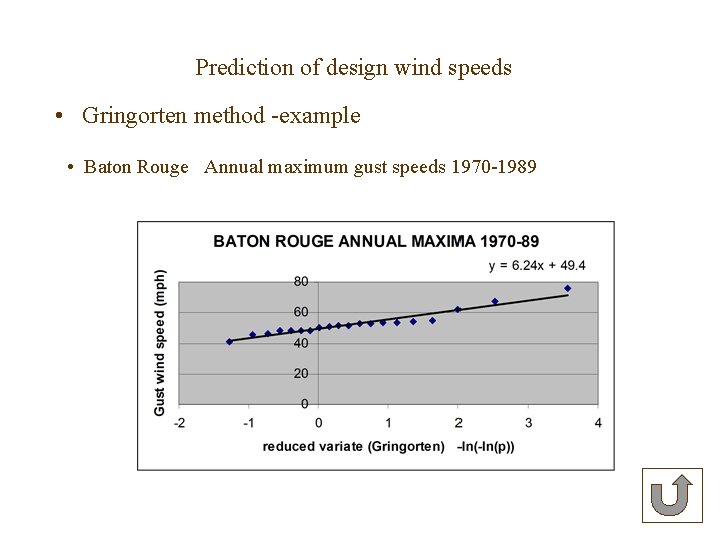
Prediction of design wind speeds • Gumbel method - for fitting Type I E. V. D. to recorded extremes - procedure • Extract largest wind speed in each year • Rank series from smallest to largest m=1, 2…. . to N • Assign probability of non-exceedence • Form reduced variate : y = - loge (-loge p) • Plot U versus y, and draw straight line of best fit, using least squares method (linear regression) for example

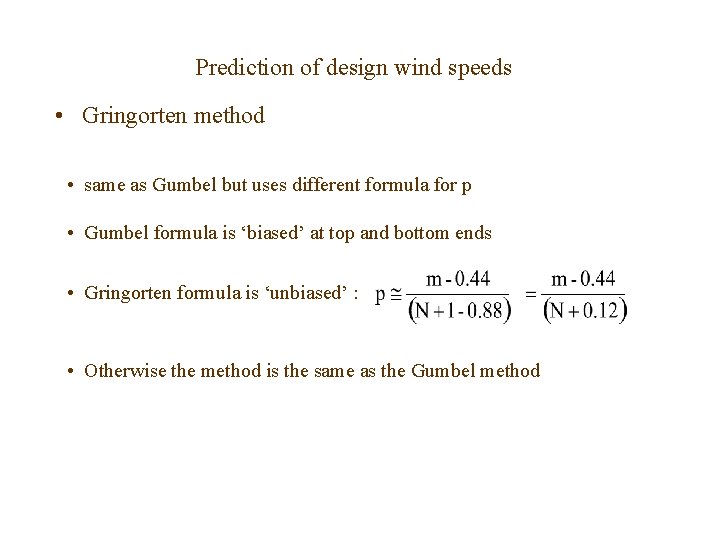
Prediction of design wind speeds • Gringorten method • same as Gumbel but uses different formula for p • Gumbel formula is ‘biased’ at top and bottom ends • Gringorten formula is ‘unbiased’ : • Otherwise the method is the same as the Gumbel method

Prediction of design wind speeds • Gumbel/ Gringorten methods - example • Baton Rouge Annual maximum gust speeds 1970 -1989 y = - loge (-loge p)

Prediction of design wind speeds • Gringorten method -example • Baton Rouge Annual maximum gust speeds 1970 -1989

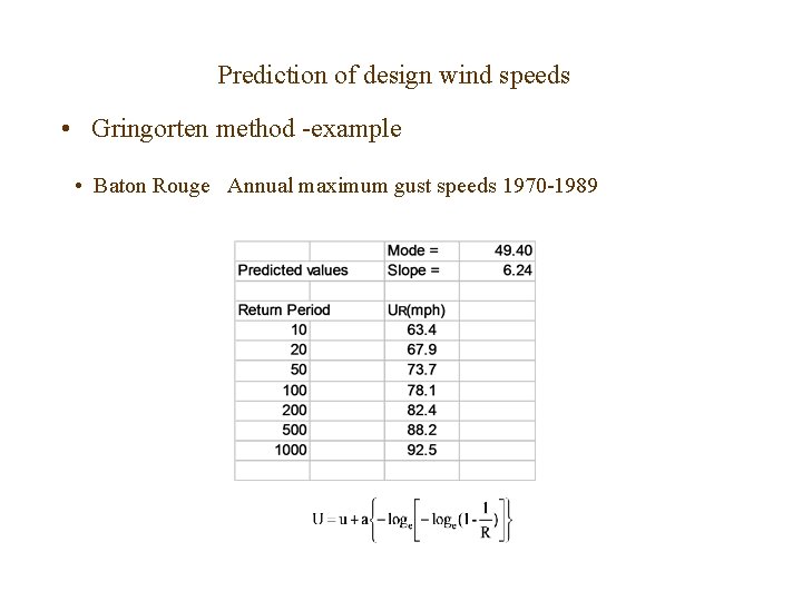
Prediction of design wind speeds • Gringorten method -example • Baton Rouge Annual maximum gust speeds 1970 -1989

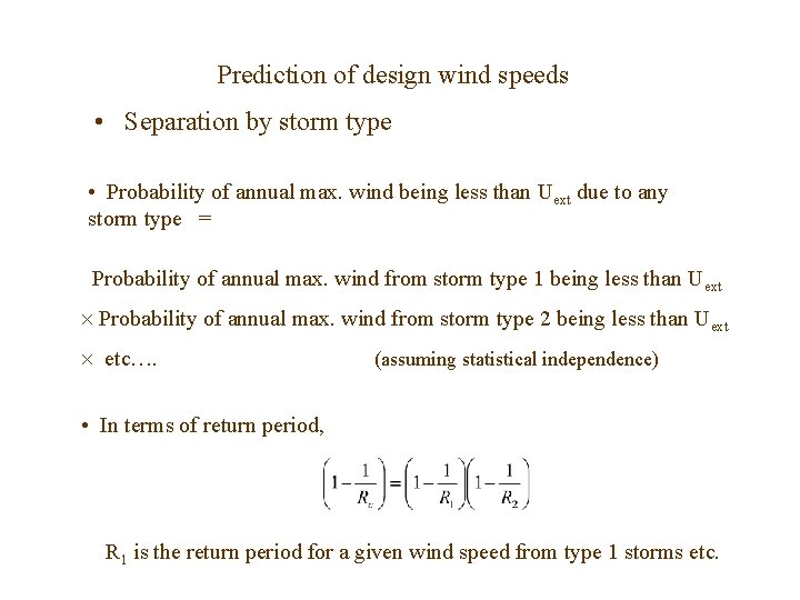
Prediction of design wind speeds • Separation by storm type • Baton Rouge data (and that from many other places) indicate a ‘mixed wind climate’ • Some annual maxima are caused by hurricanes, some by thunderstorms, some by winter gales • Effect : often an upward curvature in Gumbel/Gringorten plot • Should try to separate storm types by, for example, inspection of detailed anemometer charts, or by published hurricane tracks

Prediction of design wind speeds • Separation by storm type • Probability of annual max. wind being less than Uext due to any storm type = Probability of annual max. wind from storm type 1 being less than Uext Probability of annual max. wind from storm type 2 being less than Uext etc…. (assuming statistical independence) • In terms of return period, R 1 is the return period for a given wind speed from type 1 storms etc.

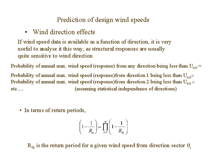
Prediction of design wind speeds • Wind direction effects If wind speed data is available as a function of direction, it is very useful to analyse it this way, as structural responses are usually quite sensitive to wind direction Probability of annual max. wind speed (response) from any direction being less than Uext = Probability of annual max. wind speed (response)from direction 1 being less than Uext Probability of annual max. wind speed (response)from direction 2 being less than Uext etc…. (assuming statistical independence of directions) • In terms of return periods, R i is the return period for a given wind speed from direction sector i

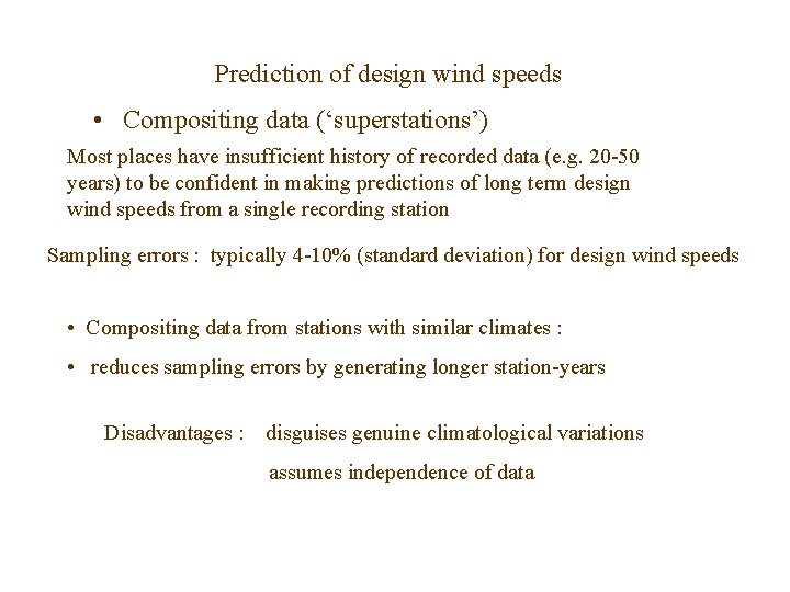
Prediction of design wind speeds • Compositing data (‘superstations’) Most places have insufficient history of recorded data (e. g. 20 -50 years) to be confident in making predictions of long term design wind speeds from a single recording station Sampling errors : typically 4 -10% (standard deviation) for design wind speeds • Compositing data from stations with similar climates : • reduces sampling errors by generating longer station-years Disadvantages : disguises genuine climatological variations assumes independence of data

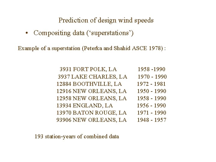
Prediction of design wind speeds • Compositing data (‘superstations’) Example of a superstation (Peterka and Shahid ASCE 1978) : 3931 FORT POLK, LA 3937 LAKE CHARLES, LA 12884 BOOTHVILLE, LA 12916 NEW ORLEANS, LA 12958 NEW ORLEANS, LA 13934 ENGLAND, LA 13970 BATON ROUGE, LA 93906 NEW ORLEANS, LA 193 station-years of combined data 1958 -1990 1970 - 1990 1972 - 1981 1950 - 1990 1958 - 1990 1956 - 1990 1971 - 1990 1948 - 1957

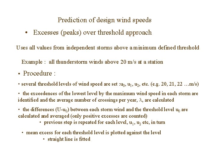
Prediction of design wind speeds • Excesses (peaks) over threshold approach Uses all values from independent storms above a minimum defined threshold Example : all thunderstorm winds above 20 m/s at a station • Procedure : • several threshold levels of wind speed are set : u 0, u 1, u 2, etc. (e. g. 20, 21, 22 …m/s) • the exceedences of the lowest level by the maximum wind speed in each storm are identified and the average number of crossings per year, , are calculated • the differences (U-u 0) between each storm wind and the threshold level u 0 are calculated and averaged (only positive excesses are counted) • previous step is repeated for each level, u 1, u 2 etc, in turn • mean excess for each threshold level is plotted against the level • straight line is fitted

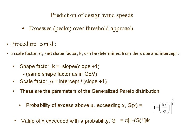
Prediction of design wind speeds • Excesses (peaks) over threshold approach • Procedure contd. : • a scale factor, , and shape factor, k, can be determined from the slope and intercept : • Shape factor, k = -slope/(slope +1) - (same shape factor as in GEV) • Scale factor, = intercept / (slope +1) • These are the parameters of the Generalized Pareto distribution • Probability of excess above uo exceeding x, G(x) = • Value of x exceeded with a probability, G = [1 -(G) k]/k

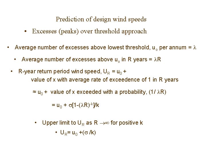
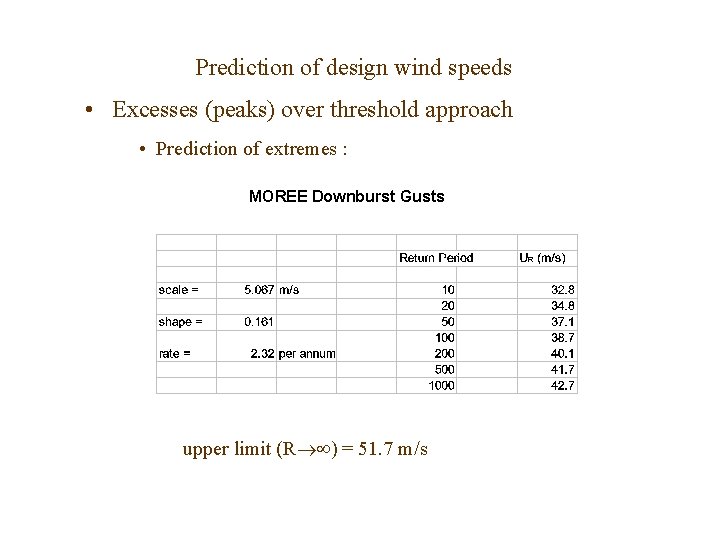
Prediction of design wind speeds • Excesses (peaks) over threshold approach • Average number of excesses above lowest threshold, uo per annum = • Average number of excesses above uo in R years = R • R-year return period wind speed, UR = u 0 + value of x with average rate of exceedence of 1 in R years ≈ u 0 + value of x exceeded with a probability, (1/ R) = u 0 + [1 -( R)-k]/k • Upper limit to UR as R for positive k • UR= u 0 +( /k)

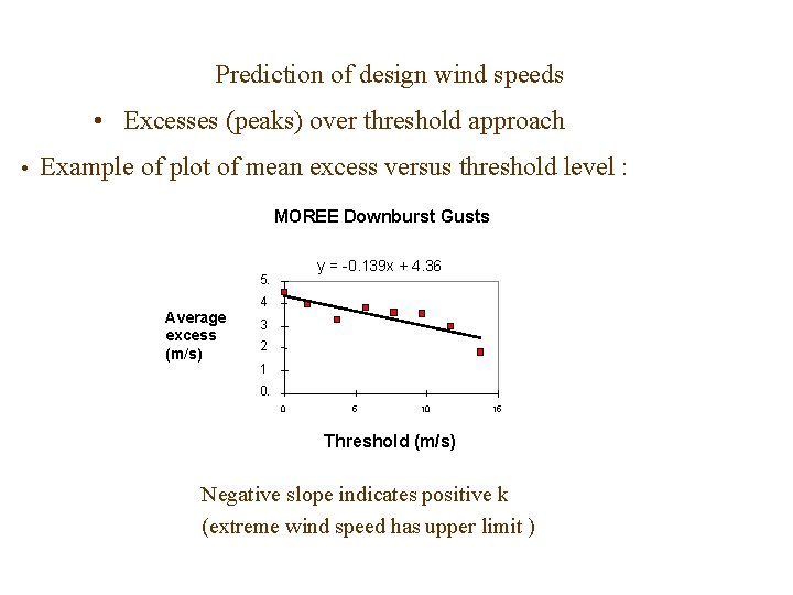
Prediction of design wind speeds • Excesses (peaks) over threshold approach • Example of plot of mean excess versus threshold level : MOREE Downburst Gusts y = -0. 139 x + 4. 36 5. Average excess (m/s) 4 3 2 1 0. 0 5 10 15 Threshold (m/s) Negative slope indicates positive k (extreme wind speed has upper limit )

Prediction of design wind speeds • Excesses (peaks) over threshold approach • Prediction of extremes : MOREE Downburst Gusts upper limit (R ) = 51. 7 m/s

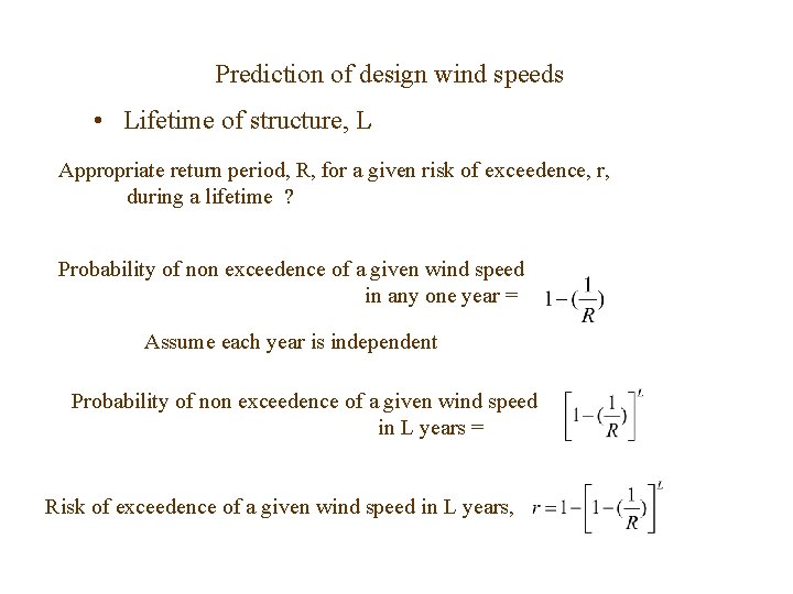
Prediction of design wind speeds • Lifetime of structure, L Appropriate return period, R, for a given risk of exceedence, r, during a lifetime ? Probability of non exceedence of a given wind speed in any one year = Assume each year is independent Probability of non exceedence of a given wind speed in L years = Risk of exceedence of a given wind speed in L years,

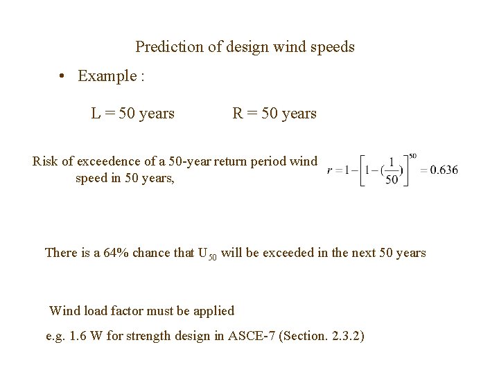
Prediction of design wind speeds • Example : L = 50 years Risk of exceedence of a 50 -year return period wind speed in 50 years, There is a 64% chance that U 50 will be exceeded in the next 50 years Wind load factor must be applied e. g. 1. 6 W for strength design in ASCE-7 (Section. 2. 3. 2)

End of Lecture 4 John Holmes 225 -405 -3789 JHolmes@bigpond. com