Warmup as you walk in https highlevel4 herokuapp

Warm-up as you walk in https: //high-level-4. herokuapp. com/experiment https: //rach 0012. github. io/human. RL_website/

Announcements Assignments: § HW 8 § Due Tue 3/26, 10 pm § P 4 § Due Thu 3/28, 10 pm § HW 9 (written) § Plan: Out tomorrow, due Tue 4/2

AI: Representation and Problem Solving Reinforcement Learning II Instructors: Pat Virtue & Stephanie Rosenthal Slide credits: CMU AI and http: //ai. berkeley. edu

Reinforcement Learning We still assume an MDP: § A set of states s S § A set of actions (per state) A § A model T(s, a, s’) § A reward function R(s, a, s’) Still looking for a policy (s) New twist: don’t know T or R, so must try out actions Big idea: Compute all averages over T using sample outcomes

Temporal Difference Learning

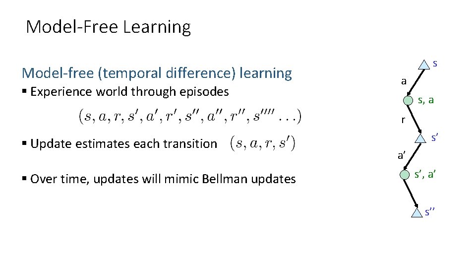
Model-Free Learning Model-free (temporal difference) learning § Experience world through episodes s a s, a r § Update estimates each transition § Over time, updates will mimic Bellman updates s’ a’ s’, a’ s’’

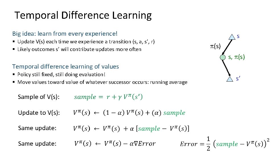
Temporal Difference Learning Big idea: learn from every experience! s § Update V(s) each time we experience a transition (s, a, s’, r) § Likely outcomes s’ will contribute updates more often (s) s, (s) Temporal difference learning of values § Policy still fixed, still doing evaluation! § Move values toward value of whatever successor occurs: running average Sample of V(s): Update to V(s): Same update: s’

Gradient Descent

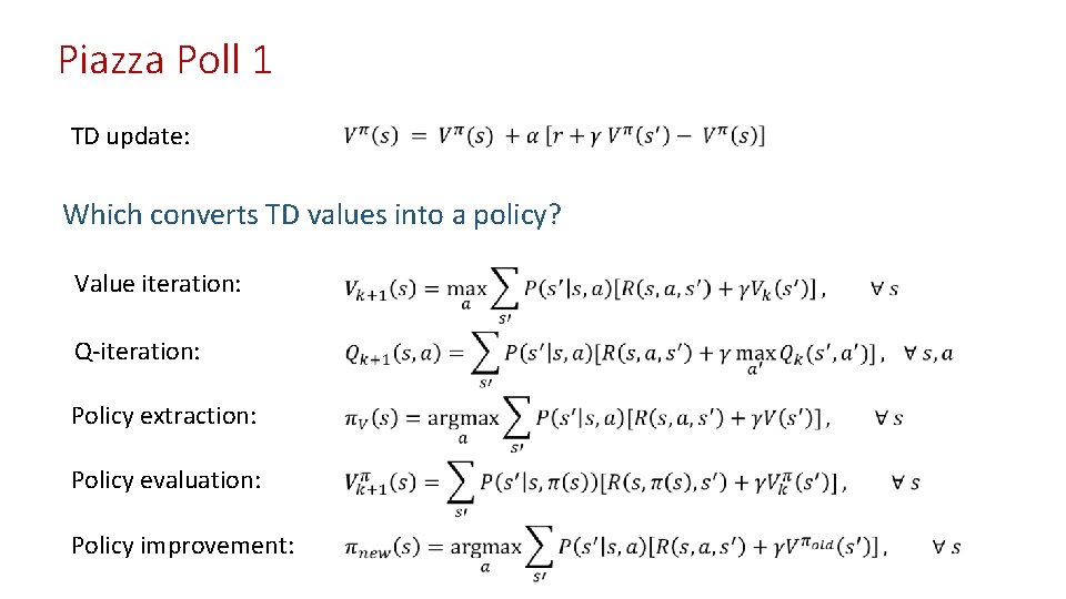
Piazza Poll 1 TD update: Which converts TD values into a policy? Value iteration: Q-iteration: Policy extraction: Policy evaluation: Policy improvement:

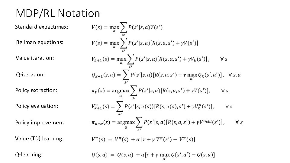
MDP/RL Notation Standard expectimax: Bellman equations: Value iteration: Q-iteration: Policy extraction: Policy evaluation: Policy improvement: Value (TD) learning: Q-learning:

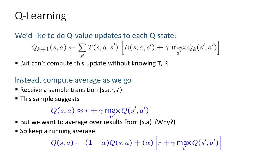
Q-Learning We’d like to do Q-value updates to each Q-state: § But can’t compute this update without knowing T, R Instead, compute average as we go § Receive a sample transition (s, a, r, s’) § This sample suggests § But we want to average over results from (s, a) (Why? ) § So keep a running average

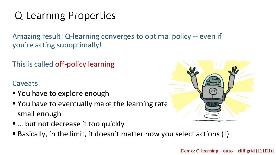
Q-Learning Properties Amazing result: Q-learning converges to optimal policy -- even if you’re acting suboptimally! This is called off-policy learning Caveats: § You have to explore enough § You have to eventually make the learning rate small enough § … but not decrease it too quickly § Basically, in the limit, it doesn’t matter how you select actions (!) [Demo: Q-learning – auto – cliff grid (L 11 D 1)]

Demo Q-Learning Auto Cliff Grid [Demo: Q-learning – auto – cliff grid (L 11 D 1)]

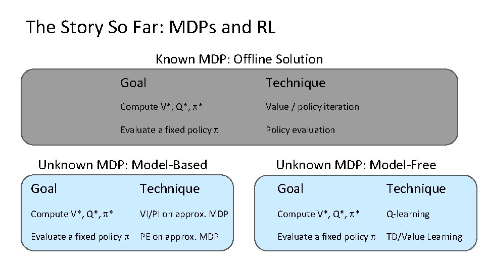
The Story So Far: MDPs and RL Known MDP: Offline Solution Goal Technique Compute V*, Q*, * Value / policy iteration Evaluate a fixed policy Policy evaluation Unknown MDP: Model-Based Unknown MDP: Model-Free Goal Technique Compute V*, Q*, * VI/PI on approx. MDP Compute V*, Q*, * Q-learning Evaluate a fixed policy PE on approx. MDP Evaluate a fixed policy TD/Value Learning

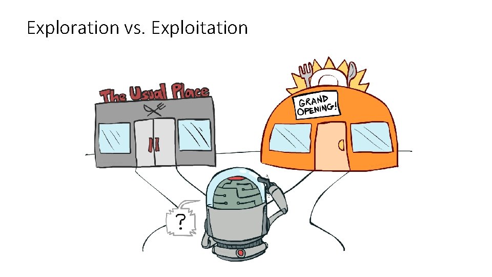
Exploration vs. Exploitation

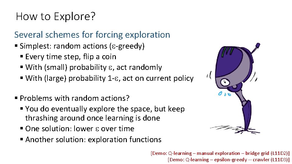
How to Explore? Several schemes forcing exploration § Simplest: random actions ( -greedy) § Every time step, flip a coin § With (small) probability , act randomly § With (large) probability 1 - , act on current policy § Problems with random actions? § You do eventually explore the space, but keep thrashing around once learning is done § One solution: lower over time § Another solution: exploration functions [Demo: Q-learning – manual exploration – bridge grid (L 11 D 2)] [Demo: Q-learning – epsilon-greedy -- crawler (L 11 D 3)]

Demo Q-learning – Manual Exploration – Bridge Grid

Demo Q-learning – Epsilon-Greedy – Crawler

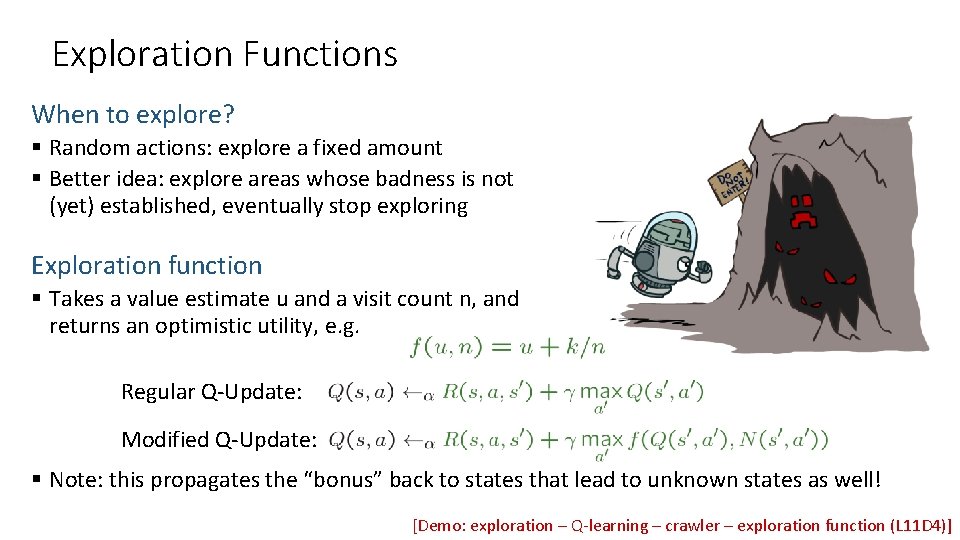
Exploration Functions When to explore? § Random actions: explore a fixed amount § Better idea: explore areas whose badness is not (yet) established, eventually stop exploring Exploration function § Takes a value estimate u and a visit count n, and returns an optimistic utility, e. g. Regular Q-Update: Modified Q-Update: § Note: this propagates the “bonus” back to states that lead to unknown states as well! [Demo: exploration – Q-learning – crawler – exploration function (L 11 D 4)]

Demo Q-learning – Exploration Function – Crawler

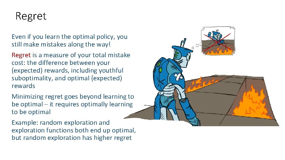
Regret Even if you learn the optimal policy, you still make mistakes along the way! Regret is a measure of your total mistake cost: the difference between your (expected) rewards, including youthful suboptimality, and optimal (expected) rewards Minimizing regret goes beyond learning to be optimal – it requires optimally learning to be optimal Example: random exploration and exploration functions both end up optimal, but random exploration has higher regret

Approximate Q-Learning

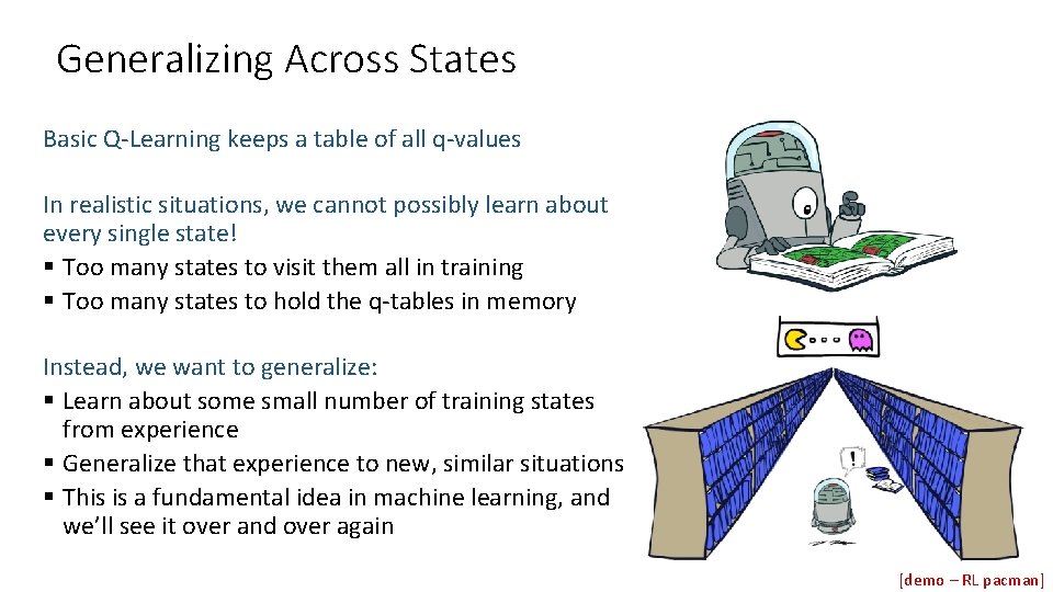
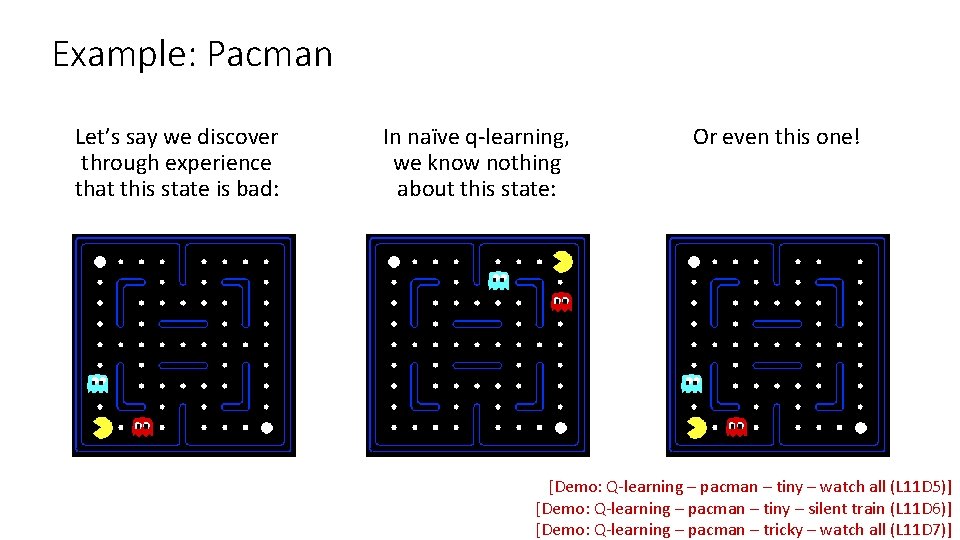
Generalizing Across States Basic Q-Learning keeps a table of all q-values In realistic situations, we cannot possibly learn about every single state! § Too many states to visit them all in training § Too many states to hold the q-tables in memory Instead, we want to generalize: § Learn about some small number of training states from experience § Generalize that experience to new, similar situations § This is a fundamental idea in machine learning, and we’ll see it over and over again [demo – RL pacman]

Example: Pacman Let’s say we discover through experience that this state is bad: In naïve q-learning, we know nothing about this state: Or even this one! [Demo: Q-learning – pacman – tiny – watch all (L 11 D 5)] [Demo: Q-learning – pacman – tiny – silent train (L 11 D 6)] [Demo: Q-learning – pacman – tricky – watch all (L 11 D 7)]

Demo Q-Learning Pacman – Tiny – Watch All

Demo Q-Learning Pacman – Tiny – Silent Train

Demo Q-Learning Pacman – Tricky – Watch All

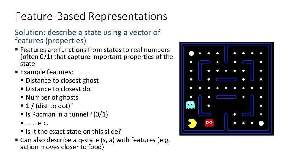
Feature-Based Representations Solution: describe a state using a vector of features (properties) § Features are functions from states to real numbers (often 0/1) that capture important properties of the state § Example features: § Distance to closest ghost § Distance to closest dot § Number of ghosts § 1 / (dist to dot)2 § Is Pacman in a tunnel? (0/1) § …… etc. § Is it the exact state on this slide? § Can also describe a q-state (s, a) with features (e. g. action moves closer to food)

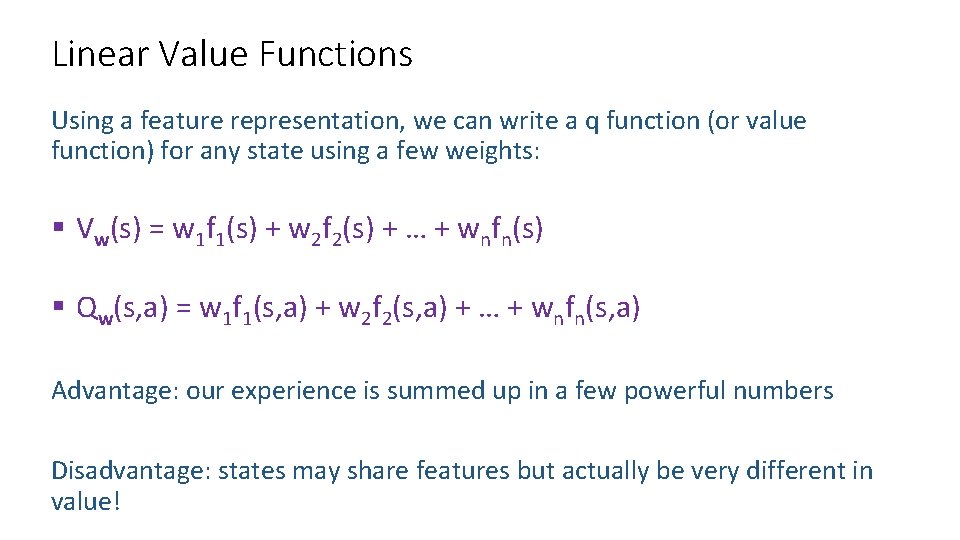
Linear Value Functions Using a feature representation, we can write a q function (or value function) for any state using a few weights: § Vw(s) = w 1 f 1(s) + w 2 f 2(s) + … + wnfn(s) § Qw(s, a) = w 1 f 1(s, a) + w 2 f 2(s, a) + … + wnfn(s, a) Advantage: our experience is summed up in a few powerful numbers Disadvantage: states may share features but actually be very different in value!

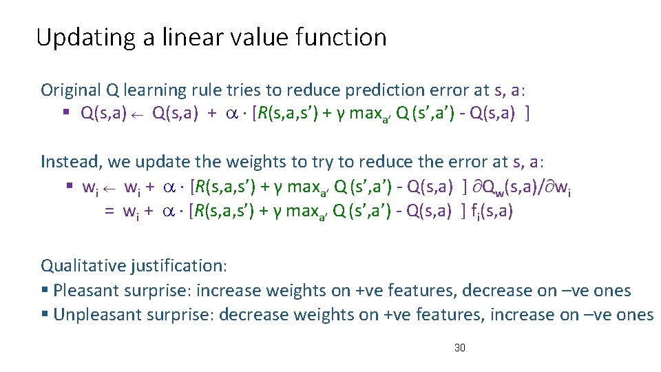
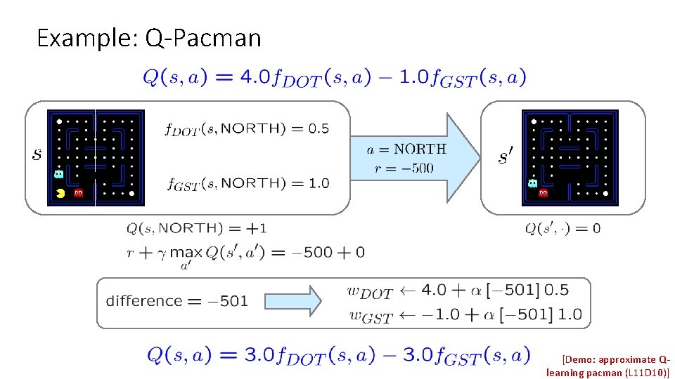
Updating a linear value function Original Q learning rule tries to reduce prediction error at s, a: § Q(s, a) + [R(s, a, s’) + γ maxa’ Q (s’, a’) - Q(s, a) ] Instead, we update the weights to try to reduce the error at s, a: § wi + [R(s, a, s’) + γ maxa’ Q (s’, a’) - Q(s, a) ] Qw(s, a)/ wi = wi + [R(s, a, s’) + γ maxa’ Q (s’, a’) - Q(s, a) ] fi(s, a) Qualitative justification: § Pleasant surprise: increase weights on +ve features, decrease on –ve ones § Unpleasant surprise: decrease weights on +ve features, increase on –ve ones 30

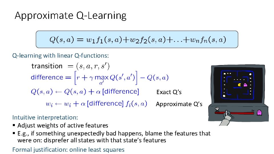
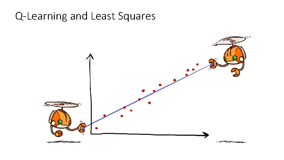
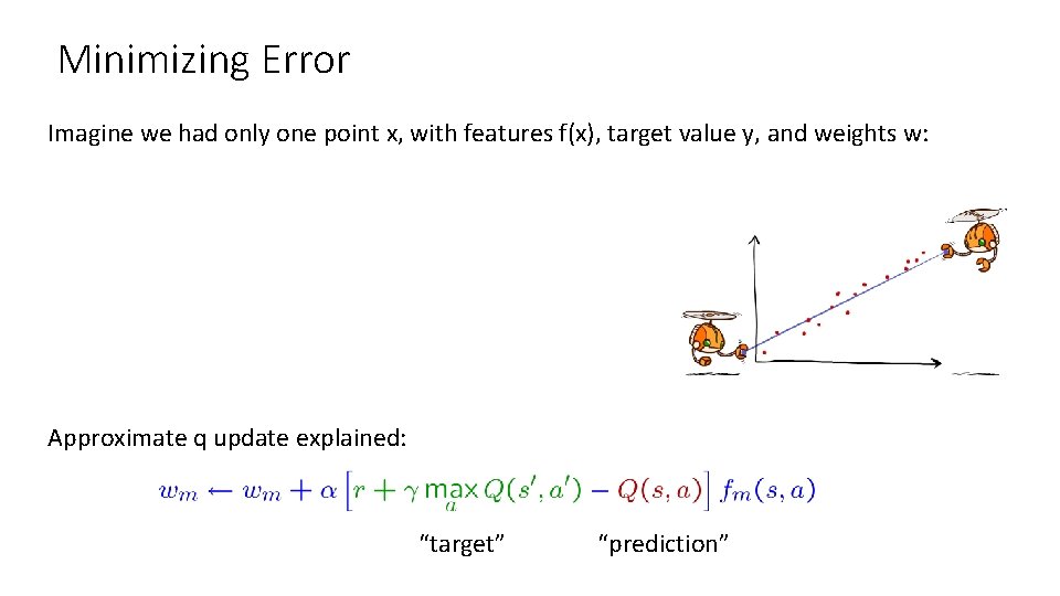
Approximate Q-Learning Q-learning with linear Q-functions: Exact Q’s Approximate Q’s Intuitive interpretation: § Adjust weights of active features § E. g. , if something unexpectedly bad happens, blame the features that were on: disprefer all states with that state’s features Formal justification: online least squares

Example: Q-Pacman [Demo: approximate Qlearning pacman (L 11 D 10)]

Demo Approximate Q-Learning -- Pacman

Q-Learning and Least Squares

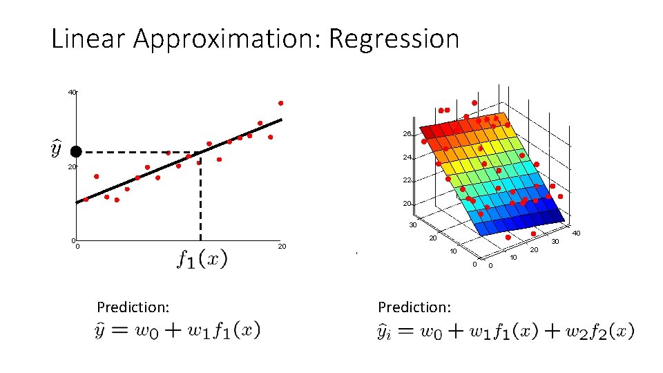
Linear Approximation: Regression 40 26 24 20 22 20 30 40 20 0 0 20 30 20 10 0 Prediction: 10 0

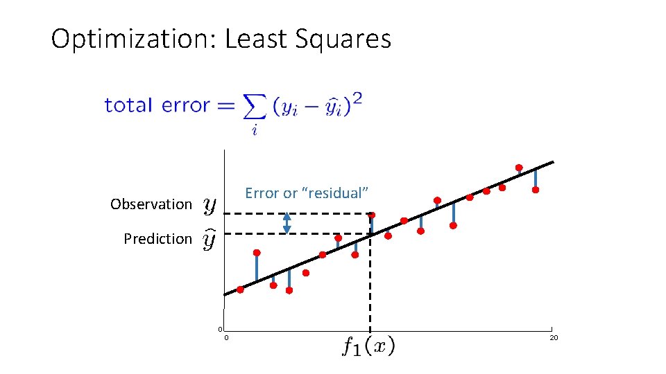
Optimization: Least Squares Error or “residual” Observation Prediction 0 0 20

Minimizing Error Imagine we had only one point x, with features f(x), target value y, and weights w: Approximate q update explained: “target” “prediction”

Recent Reinforcement Learning Milestones

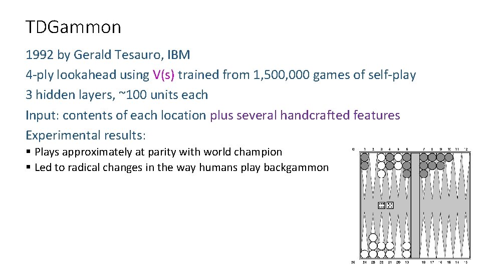
TDGammon 1992 by Gerald Tesauro, IBM 4 -ply lookahead using V(s) trained from 1, 500, 000 games of self-play 3 hidden layers, ~100 units each Input: contents of each location plus several handcrafted features Experimental results: § Plays approximately at parity with world champion § Led to radical changes in the way humans play backgammon

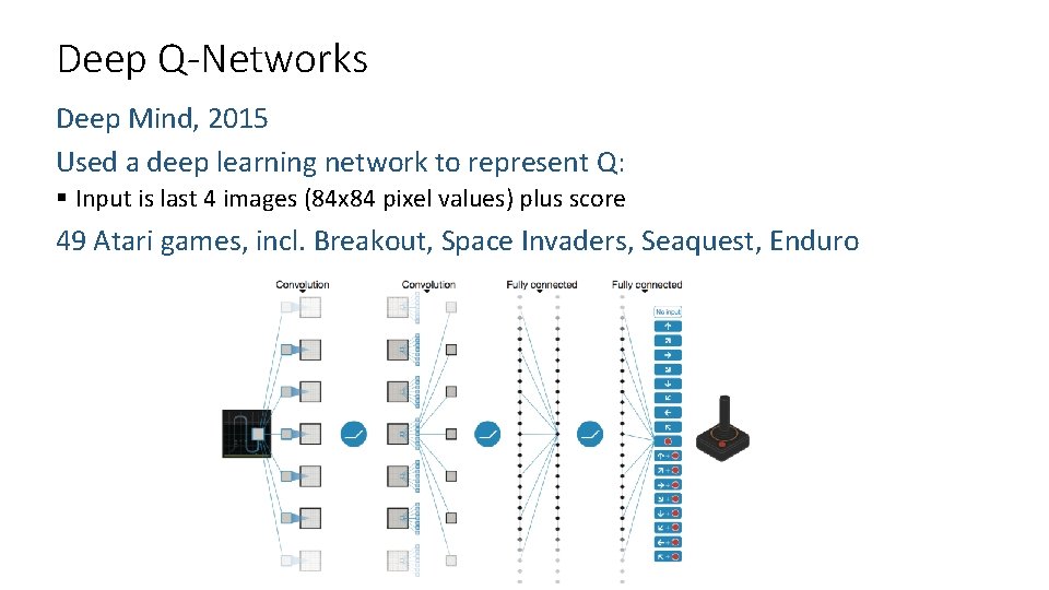
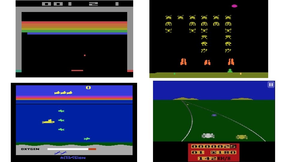
Deep Q-Networks Deep Mind, 2015 Used a deep learning network to represent Q: § Input is last 4 images (84 x 84 pixel values) plus score 49 Atari games, incl. Breakout, Space Invaders, Seaquest, Enduro 40

41

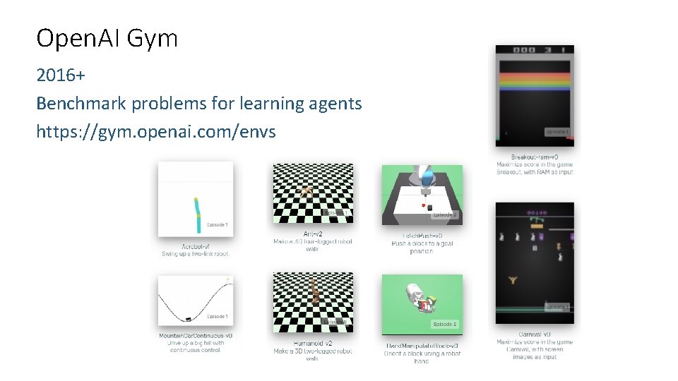
Open. AI Gym 2016+ Benchmark problems for learning agents https: //gym. openai. com/envs

Alpha. Go, Alpha. Zero Deep Mind, 2016+

Autonomous Vehicles?