Twenty Second Annual Meeting 20192020 Multivariate Analysis for

Twenty Second Annual Meeting: 2019/2020 Multivariate Analysis for Response Surface Methodology: Horn River Shale Case Study Chuks Anthony Sunday

Content • Introduction • Objective • Methodology • Data structure • Exploratory data analysis • Data Imputation • Response Surface Methodology (RSM) • Conclusions • References 2

Introduction • Multiple geological rock properties are jointly used for characterizing geologic deposits of formation • Geological and engineering models are constructed from multiple rock properties • Geological models – to assess resources/reserves • Engineering models - for engineering design, study and optimize processes, and for predictions of properties of interest • Multivariate analysis and property modeling are thus very essential in resource management 3

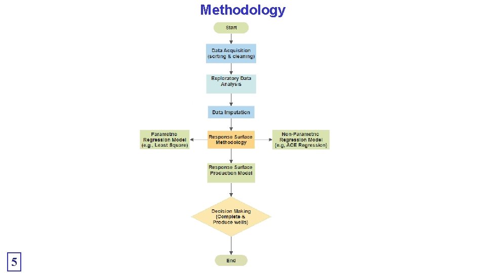
Objectives • Understand the multivariate relationships between the HRS formation properties • Use both parametric and non-parametric response surface methodologies (RSM) to develop response surface production models for the HRS formation. 4

Methodology 5

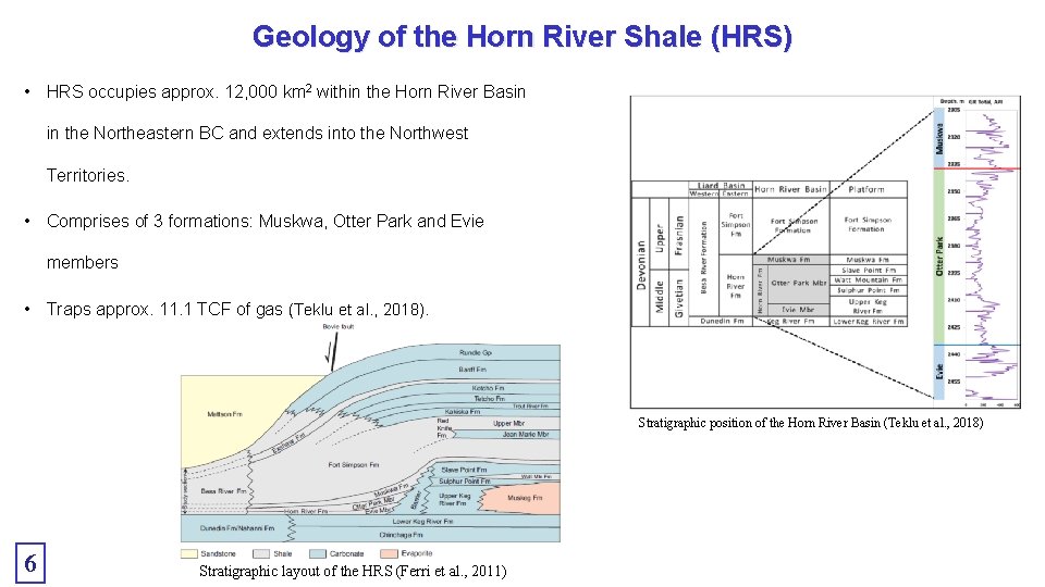
Geology of the Horn River Shale (HRS) • HRS occupies approx. 12, 000 km 2 within the Horn River Basin in the Northeastern BC and extends into the Northwest Territories. • Comprises of 3 formations: Muskwa, Otter Park and Evie members • Traps approx. 11. 1 TCF of gas (Teklu et al. , 2018). Stratigraphic position of the Horn River Basin (Teklu et al. , 2018) 6 Stratigraphic layout of the HRS (Ferri et al. , 2011)

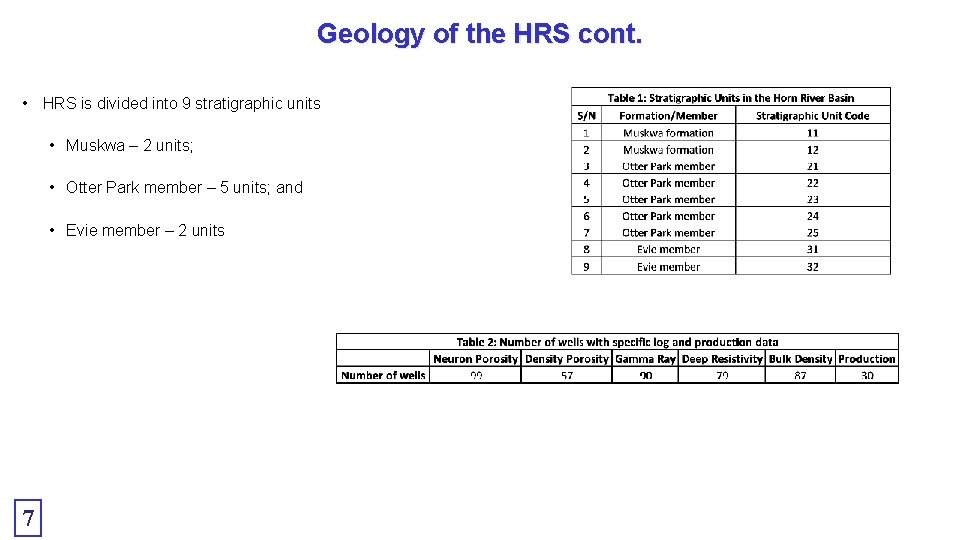
Geology of the HRS cont. • HRS is divided into 9 stratigraphic units • Muskwa – 2 units; • Otter Park member – 5 units; and • Evie member – 2 units 7

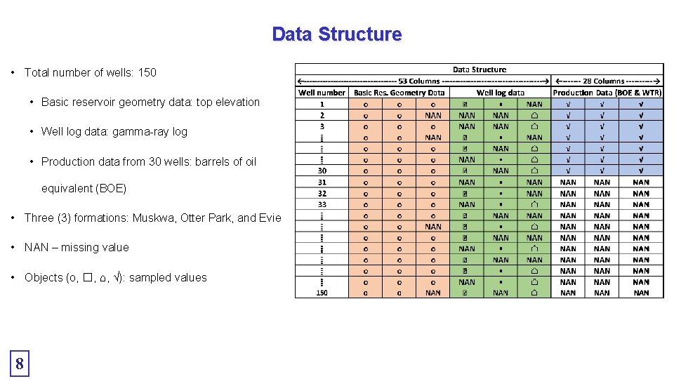
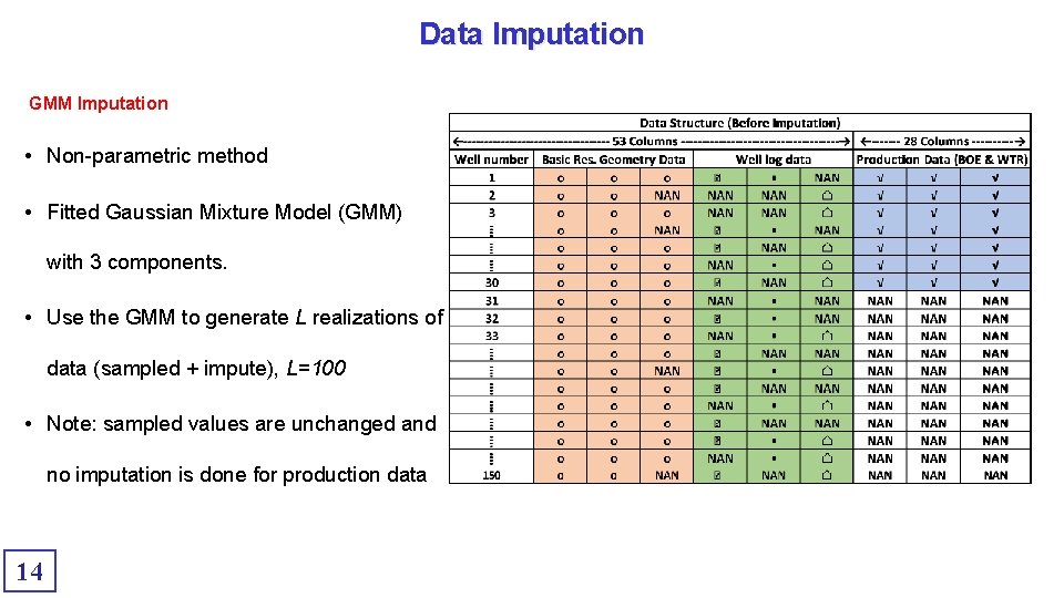
Data Structure • Total number of wells: 150 • Basic reservoir geometry data: top elevation • Well log data: gamma-ray log • Production data from 30 wells: barrels of oil equivalent (BOE) • Three (3) formations: Muskwa, Otter Park, and Evie • NAN – missing value • Objects (ᴏ, �, ⌂, √): sampled values 8

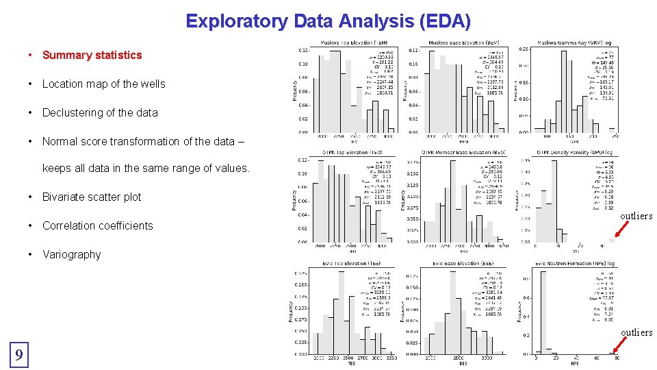
Exploratory Data Analysis (EDA) • Summary statistics • Location map of the wells • Declustering of the data • Normal score transformation of the data – keeps all data in the same range of values. • Bivariate scatter plot • Correlation coefficients outliers • Variography outliers 9

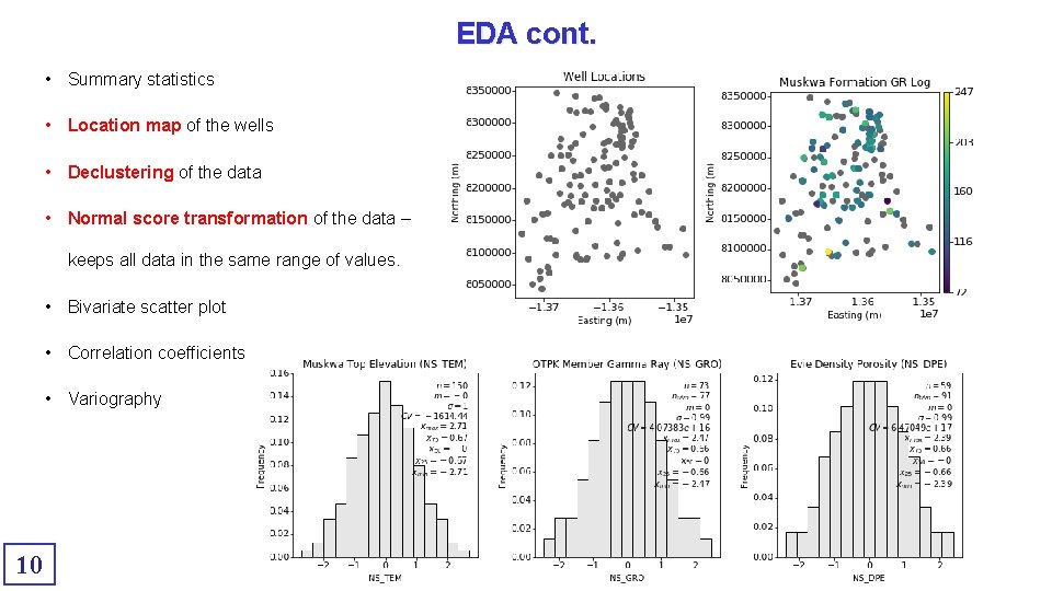
EDA cont. • Summary statistics • Location map of the wells • Declustering of the data • Normal score transformation of the data – keeps all data in the same range of values. • Bivariate scatter plot • Correlation coefficients • Variography 10

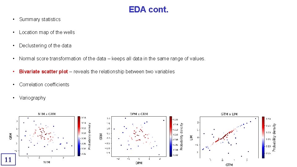
EDA cont. • Summary statistics • Location map of the wells • Declustering of the data • Normal score transformation of the data – keeps all data in the same range of values. • Bivariate scatter plot – reveals the relationship between two variables • Correlation coefficients • Variography 11

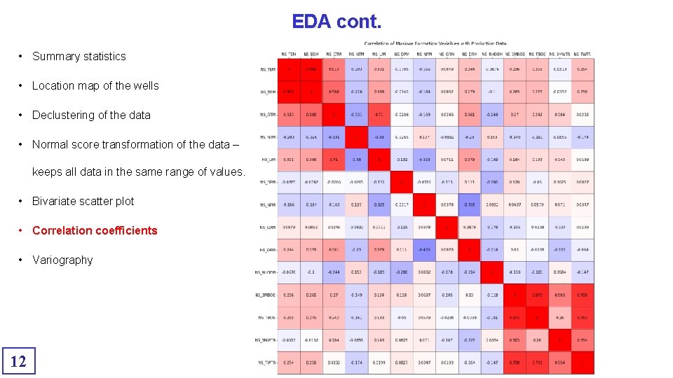
EDA cont. • Summary statistics • Location map of the wells • Declustering of the data • Normal score transformation of the data – keeps all data in the same range of values. • Bivariate scatter plot • Correlation coefficients • Variography 12

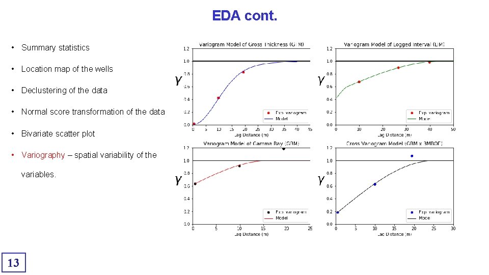
EDA cont. • Summary statistics • Location map of the wells • Declustering of the data • Normal score transformation of the data • Bivariate scatter plot • Variography – spatial variability of the variables. 13

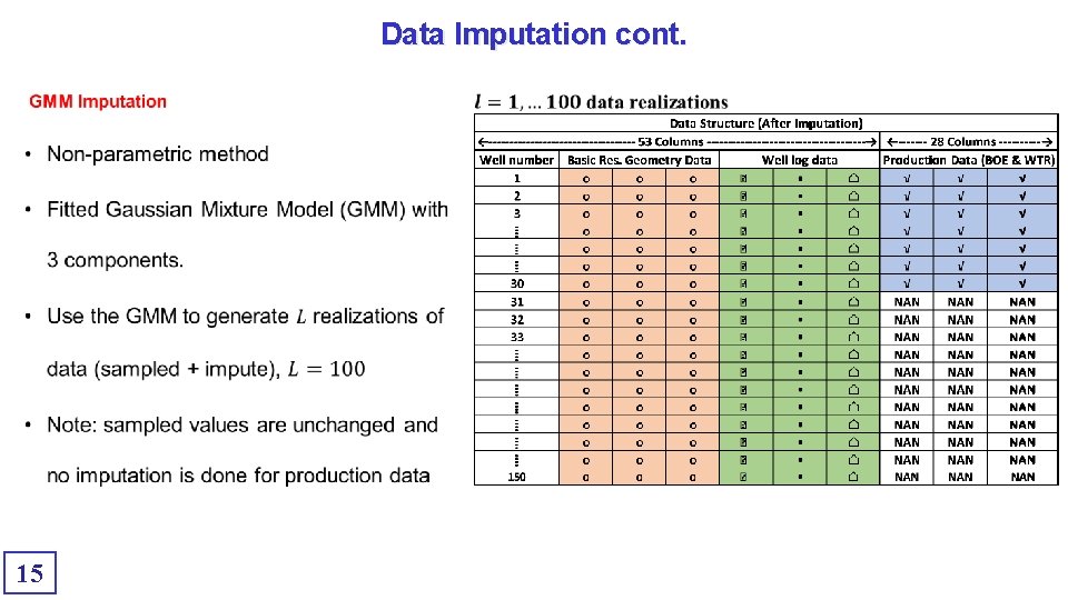
Data Imputation GMM Imputation • Non-parametric method • Fitted Gaussian Mixture Model (GMM) with 3 components. • Use the GMM to generate L realizations of data (sampled + impute), L=100 • Note: sampled values are unchanged and no imputation is done for production data 14

Data Imputation cont. • 15

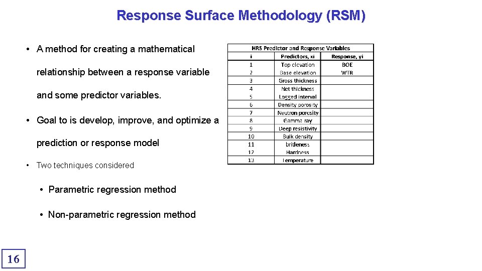
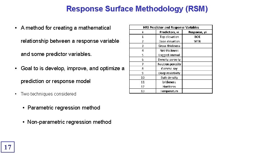
Response Surface Methodology (RSM) • A method for creating a mathematical relationship between a response variable and some predictor variables. • Goal to is develop, improve, and optimize a prediction or response model • Two techniques considered • Parametric regression method • Non-parametric regression method 16

Response Surface Methodology (RSM) • A method for creating a mathematical relationship between a response variable and some predictor variables. • Goal to is develop, improve, and optimize a prediction or response model • Two techniques considered • Parametric regression method • Non-parametric regression method 17

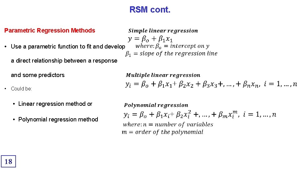
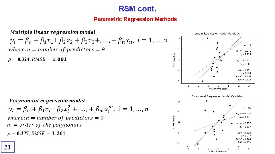
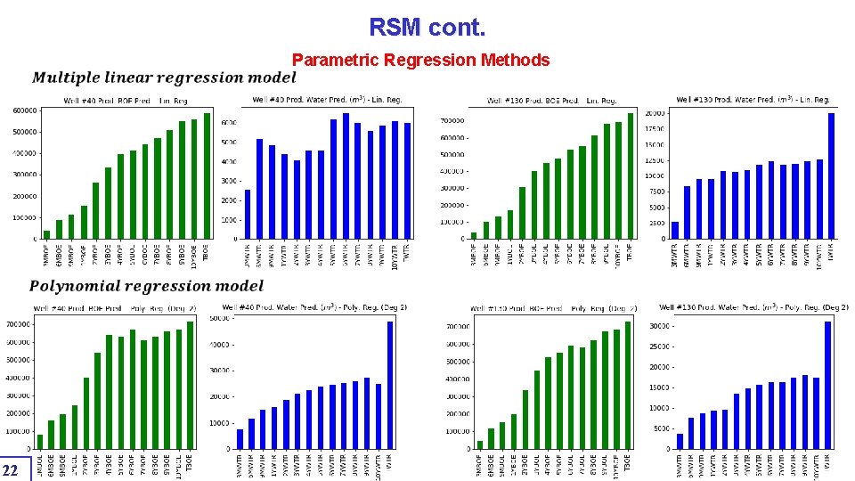
RSM cont. Parametric Regression Methods • Use a parametric function to fit and develop a direct relationship between a response and some predictors • Could be: • Linear regression method or • Polynomial regression method 18

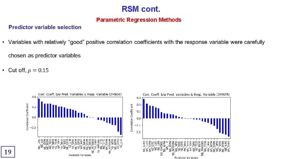
RSM cont. Parametric Regression Methods 19

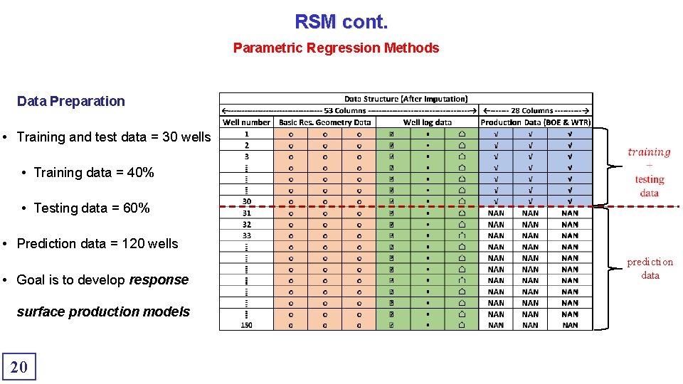
RSM cont. Parametric Regression Methods Data Preparation • Training and test data = 30 wells • Training data = 40% • Testing data = 60% • Prediction data = 120 wells • Goal is to develop response surface production models 20 prediction data

RSM cont. Parametric Regression Methods 21

RSM cont. Parametric Regression Methods 22

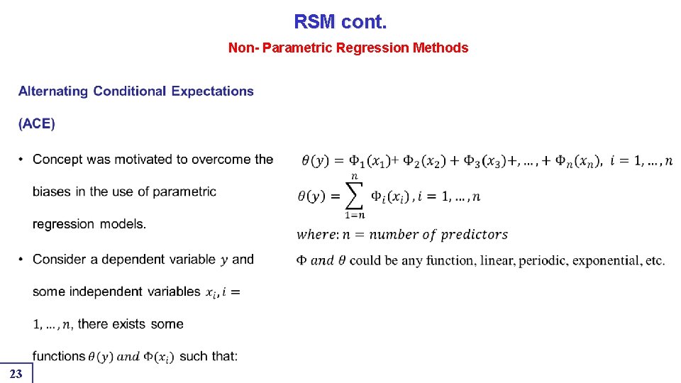
RSM cont. Non- Parametric Regression Methods 23

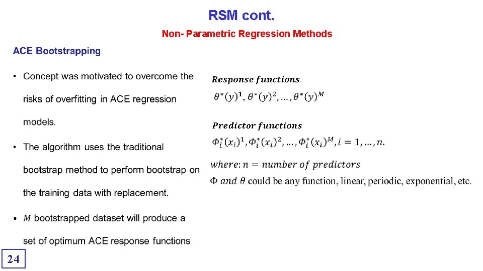
RSM cont. Non- Parametric Regression Methods 24

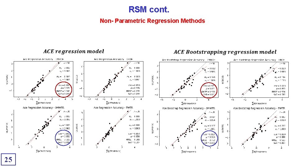
RSM cont. Non- Parametric Regression Methods 25

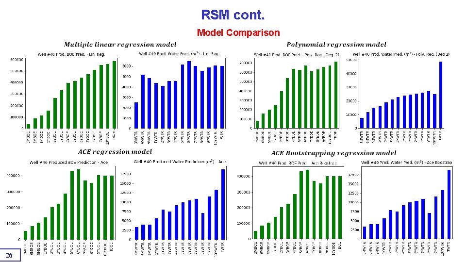
RSM cont. Model Comparison 26

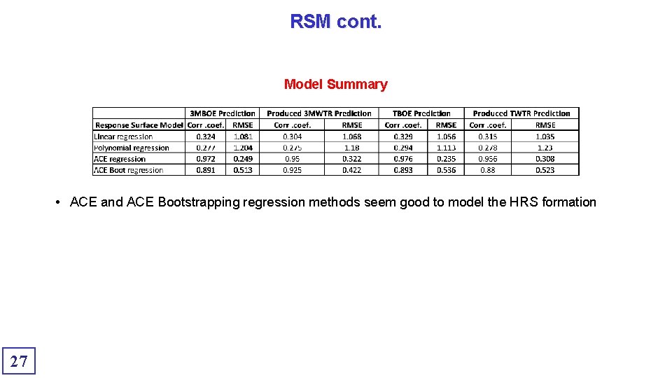
RSM cont. Model Summary • ACE and ACE Bootstrapping regression methods seem good to model the HRS formation 27

Conclusions • Parametric response surface models are easy to develop for multiple variables but are biased with non-parametric signals. • Non-parametric regression method should be used to model multiple variables with non-linear, non-parametric relationships, such as the HRS dataset. • The ACE bootstrapping regression model would yield reliable predictions since it accounts for uncertainty in the training data and is not overfitted. • Models could be used as decision making tools 28

References • Aydar, A. Y. (2018). Utilization of Response Surface Methodology in Optimization of Extraction of Plant Materials. DOI: 10. 5772/intechopen. 73690, Intechopen, https: //www. intechopen. com/books/statistical-approaches-with-emphasis-on-design-ofexperiments-applied-to-chemical-processes/utilization-of-response-surface-methodology-in-optimization-of-extraction-of-plantmaterials , February 7. • Ferri, F. , Hickin, A. , and Huntley, D. (2011). Besa River Formation, Western Liard Basin, British Columbia (NTS 094 N): Chemistry and Regional Correlations. Geoscience Reports. British Columbia Ministry of Energy, Mines and Natural Gas. • Hmoud, S. and Boisvert, J. (2016). Horn River Shale: Dataset Overview and Spatial Statistics. CCG Paper 2016 -211, Centre for Computational Geostatistics, University of Alberta, Edmonton, Canada. • Lekou, D. J. (2013). Probabilistic Design of Wind Turbine Blades – Advances in Wind Turbine Blade Design and Materials. Science. Direct, https: //www. sciencedirect. com/topics/engineering/response-surface-method • Teklu, T. W. , Park, D. , Jung, H. , and Miskimins, J. L. (2018). Integrated Rock Characterization of a Shale Gas Field in the Horn River Basin, Canada. URTe. C-2880467, presented at the Unconventional Resources Technology Conference held in Houston, Texas, USA, July 23 -25. 29

This presentation and the associated papers and software for the sole use of CCG members. Selected papers from this report may be distributed to non-members for the purpose of promoting CCG research. The report may be circulated within CCG member organizations; however, the following copyright notice must be adhered to. Copyright, 2020, Centre for Computational Geostatistics All rights reserved. No part of this presentation may be used or reproduced without written permission, except for members of the Centre for Computational Geostatistics.