Twenty Second Annual Meeting 20192020 Grade Density and

Twenty Second Annual Meeting: 2019/2020 Grade, Density, and Volume Uncertainty of the Arrow Deposit. Matt Batty

Outline • Overview of the Arrow Uranium Deposit • Study Domain • Density and Grade Uncertainty • Multivariate Spatial Bootstrap • Geometry Imputation and Volume Uncertainty • Future Study Opportunities 2

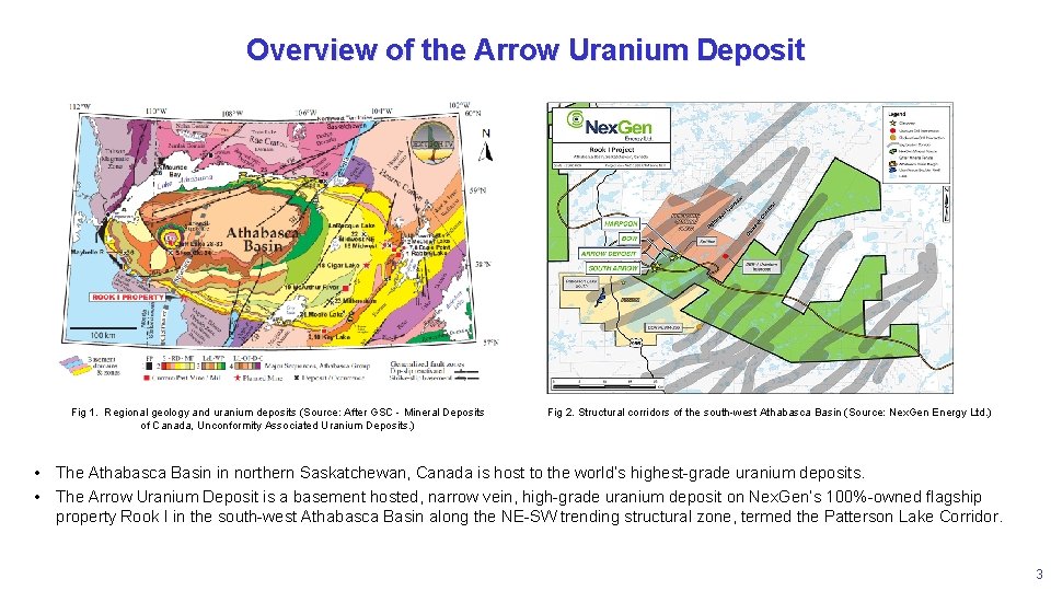
Overview of the Arrow Uranium Deposit Fig 1. Regional geology and uranium deposits (Source: After GSC - Mineral Deposits of Canada, Unconformity Associated Uranium Deposits. ) Fig 2. Structural corridors of the south-west Athabasca Basin (Source: Nex. Gen Energy Ltd. ) • The Athabasca Basin in northern Saskatchewan, Canada is host to the world’s highest-grade uranium deposits. • The Arrow Uranium Deposit is a basement hosted, narrow vein, high-grade uranium deposit on Nex. Gen’s 100%-owned flagship property Rook I in the south-west Athabasca Basin along the NE-SW trending structural zone, termed the Patterson Lake Corridor. 3

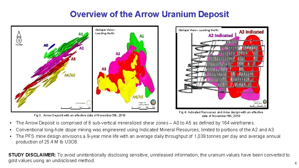
Overview of the Arrow Uranium Deposit Oblique View – Looking North Fig 3. Arrow Deposit with an effective date of November 5 th, 2018 Oblique View – Looking North Fig 4. Indicated Resources and mine design with an effective date of November 5 th, 2018 • The Arrow Deposit is comprised of 6 sub-vertical mineralized shear zones – A 0 to A 5 as defined by 164 wireframes. • Conventional long-hole stope mining was engineered using Indicated Mineral Resources; limited to portions of the A 2 and A 3. • The PFS mine design envisions a 9 -year mine life with an average daily throughput of 1, 039 tonnes per day and average annual production of 25. 4 M lb U 3 O 8. STUDY DISCLAIMER: To avoid unintentionally disclosing sensitive, unreleased information, the uranium values have been converted to gold values using an undisclosed method. 4

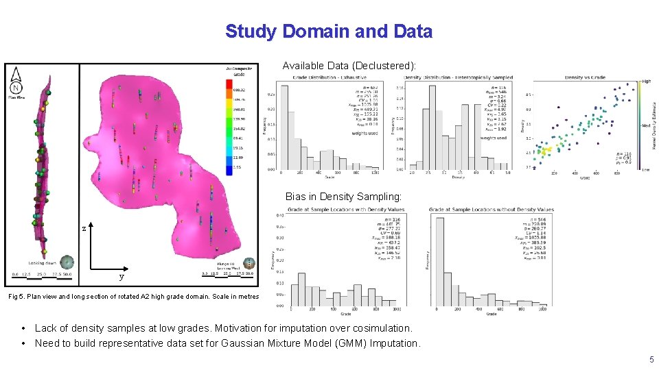
Study Domain and Data Available Data (Declustered): Bias in Density Sampling: z y Fig 5. Plan view and long section of rotated A 2 high grade domain. Scale in metres • Lack of density samples at low grades. Motivation for imputation over cosimulation. • Need to build representative data set for Gaussian Mixture Model (GMM) Imputation. 5

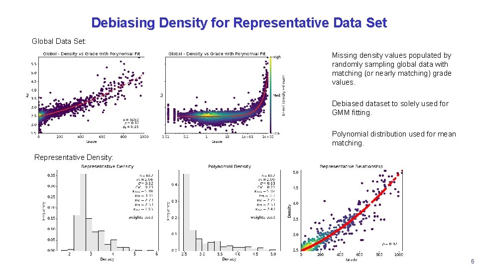
Debiasing Density for Representative Data Set Global Data Set: Missing density values populated by randomly sampling global data with matching (or nearly matching) grade values. Debiased dataset to solely used for GMM fitting. Polynomial distribution used for mean matching. Representative Density: 6

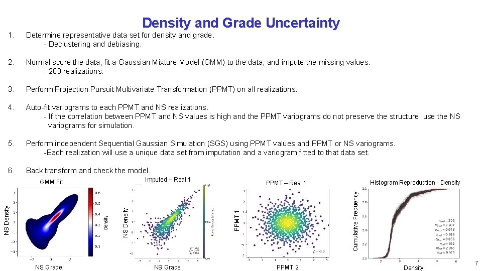
Density and Grade Uncertainty 1. Determine representative data set for density and grade. - Declustering and debiasing. 2. Normal score the data, fit a Gaussian Mixture Model (GMM) to the data, and impute the missing values. - 200 realizations. 3. Perform Projection Pursuit Multivariate Transformation (PPMT) on all realizations. 4. Auto-fit variograms to each PPMT and NS realizations. - If the correlation between PPMT and NS values is high and the PPMT variograms do not preserve the structure, use the NS variograms for simulation. 5. Perform independent Sequential Gaussian Simulation (SGS) using PPMT values and PPMT or NS variograms. -Each realization will use a unique data set from imputation and a variogram fitted to that data set. 6. Back transform and check the model. Imputed – Real 1 NS Grade Histogram Reproduction - Density Cumulative Frequency PPMT – Real 1 PPMT 1 NS Density GMM Fit PPMT 2 Density 7

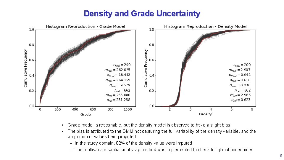
Density and Grade Uncertainty • Grade model is reasonable, but the density model is observed to have a slight bias. • The bias is attributed to the GMM not capturing the full variability of the density variable, and the proportion of values being imputed. – In the study domain, 82% of the density value were imputed. – The multivariate spatial bootstrap method was implemented to check for global uncertainty. 8

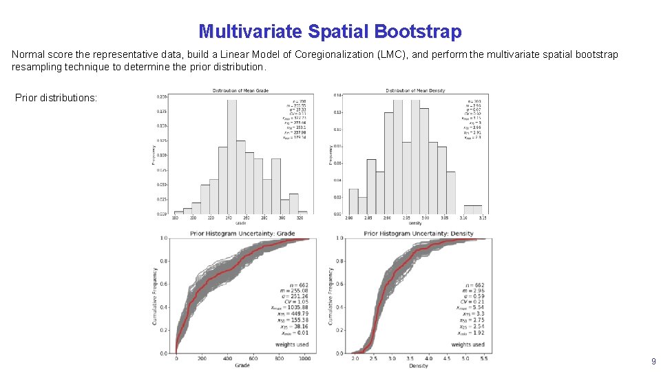
Multivariate Spatial Bootstrap Normal score the representative data, build a Linear Model of Coregionalization (LMC), and perform the multivariate spatial bootstrap resampling technique to determine the prior distribution. Prior distributions: 9

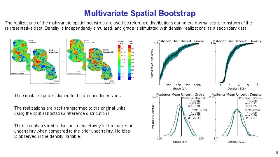
Multivariate Spatial Bootstrap The realizations of the multivariate spatial bootstrap are used as reference distributions during the normal score transform of the representative data. Density is independently simulated, and grade is simulated with density realizations as a secondary data. The simulated grid is clipped to the domain dimensions. The realizations are back transformed to the original units using the spatial bootstrap reference distributions. There is only a slight reduction in uncertainty for the posterior uncertainty when compared to the prior uncertainty. No bias is observed in the density variable. 10

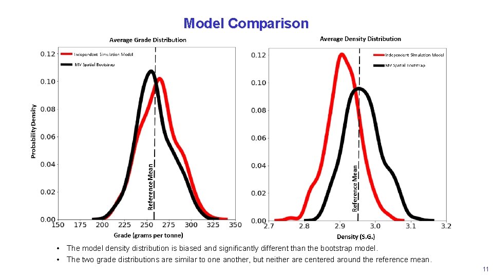
Model Comparison • The model density distribution is biased and significantly different than the bootstrap model. • The two grade distributions are similar to one another, but neither are centered around the reference mean. 11

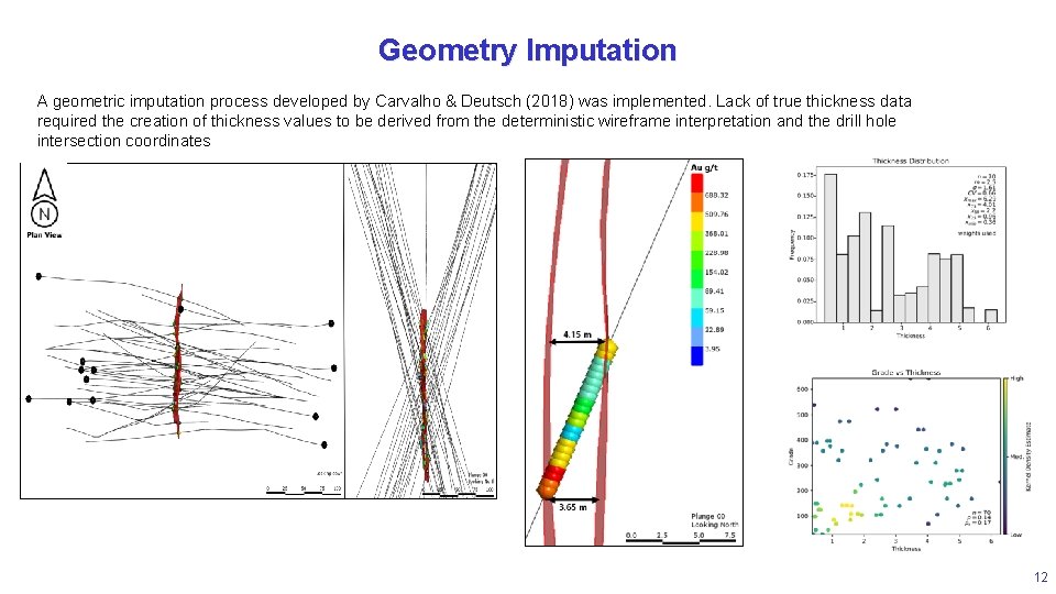
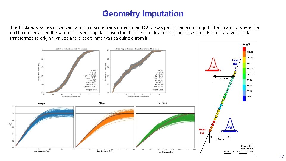
Geometry Imputation A geometric imputation process developed by Carvalho & Deutsch (2018) was implemented. Lack of true thickness data required the creation of thickness values to be derived from the deterministic wireframe interpretation and the drill hole intersection coordinates 12

Geometry Imputation The thickness values underwent a normal score transformation and SGS was performed along a grid. The locations where the drill hole intersected the wireframe were populated with the thickness realizations of the closest block. The data was back transformed to original values and a coordinate was calculated from it. 13

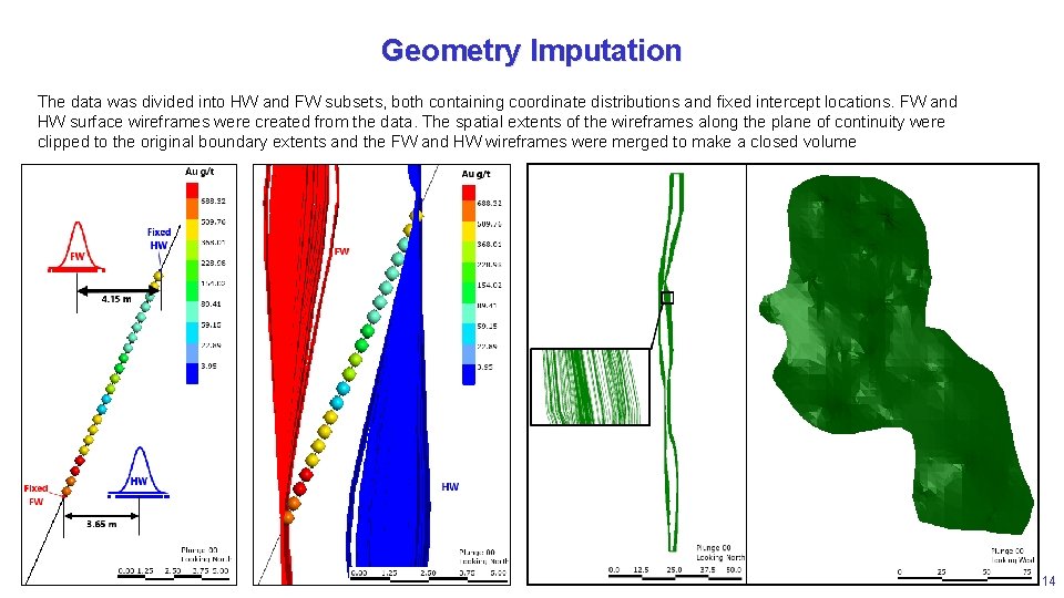
Geometry Imputation The data was divided into HW and FW subsets, both containing coordinate distributions and fixed intercept locations. FW and HW surface wireframes were created from the data. The spatial extents of the wireframes along the plane of continuity were clipped to the original boundary extents and the FW and HW wireframes were merged to make a closed volume 14

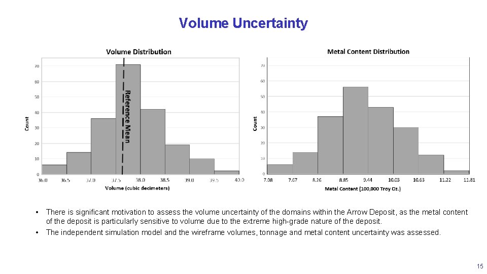
Volume Uncertainty • There is significant motivation to assess the volume uncertainty of the domains within the Arrow Deposit, as the metal content of the deposit is particularly sensitive to volume due to the extreme high-grade nature of the deposit. • The independent simulation model and the wireframe volumes, tonnage and metal content uncertainty was assessed. 15

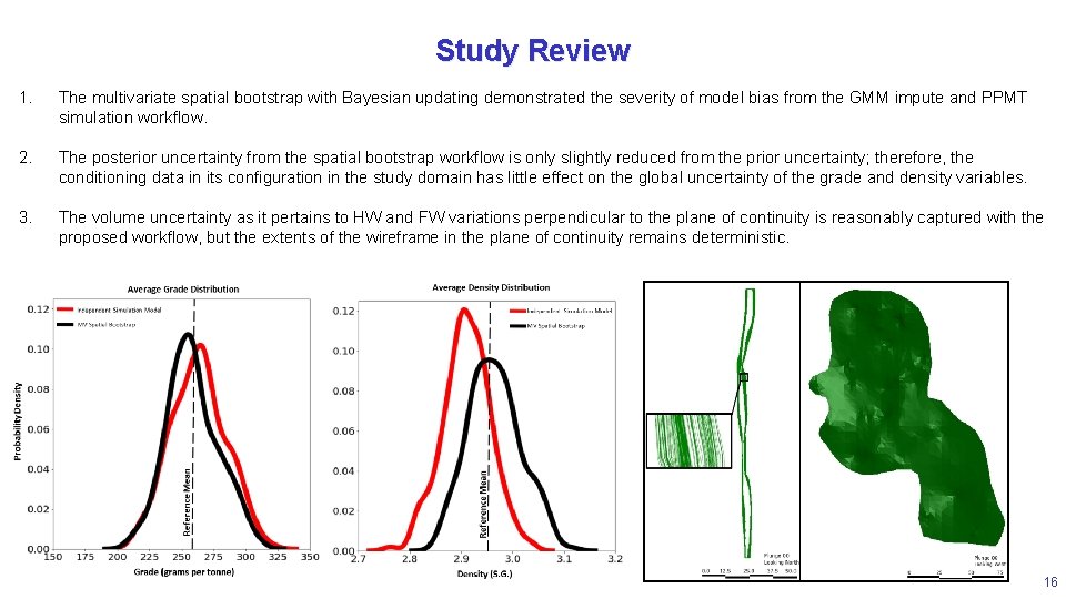
Study Review 1. The multivariate spatial bootstrap with Bayesian updating demonstrated the severity of model bias from the GMM impute and PPMT simulation workflow. 2. The posterior uncertainty from the spatial bootstrap workflow is only slightly reduced from the prior uncertainty; therefore, the conditioning data in its configuration in the study domain has little effect on the global uncertainty of the grade and density variables. 3. The volume uncertainty as it pertains to HW and FW variations perpendicular to the plane of continuity is reasonably captured with the proposed workflow, but the extents of the wireframe in the plane of continuity remains deterministic. 16

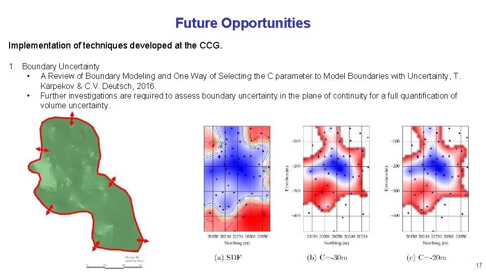
Future Opportunities Implementation of techniques developed at the CCG. 1. Boundary Uncertainty • A Review of Boundary Modeling and One Way of Selecting the C parameter to Model Boundaries with Uncertainty, T. Karpekov & C. V. Deutsch, 2016. • Further investigations are required to assess boundary uncertainty in the plane of continuity for a full quantification of volume uncertainty. 17

Future Opportunities Implementation of techniques developed at the CCG. 2. Stope Optimization. • Algorithm for Stochastic Stope Optimization, Brandon Wilson, 2018. 3. Geostatistical Modeling of Geometallugical Variables. • Geostatistical Modelling of Geometallurgical Variables - Problems and Solutions, C. V. Deustch, 2013. 18

End Thanks you for your time! Questions are encouraged. 19

This presentation and the associated papers and software for the sole use of CCG members. Selected papers from this report may be distributed to non-members for the purpose of promoting CCG research. The report may be circulated within CCG member organizations; however, the following copyright notice must be adhered to. Copyright, 2020, Centre for Computational Geostatistics All rights reserved. No part of this presentation may be used or reproduced without written permission, except for members of the Centre for Computational Geostatistics. 20