Trends in the NCARNCEP CDAS Reanalysis data Are

Trends in the NCAR/NCEP CDAS Reanalysis data: Are They Real? Vernon E. Kousky NOAA/ Climate Prediction Center 16 October 2003

Decadal Trends in CDAS/Reanalysis Questions? ? ? • Are the trends real? • Are they due to non-homogeneities in the observational data sets? • Are they partly real and partly due to nonhomogeneities in the observational data sets? Future reanalysis efforts should attempt to answer these questions.

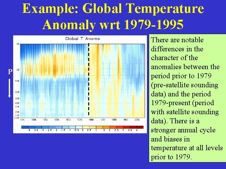
Example: Global Temperature Anomaly wrt 1979 -1995 P There are notable differences in the character of the anomalies between the period prior to 1979 (pre-satellite sounding data) and the period 1979 -present (period with satellite sounding data). There is a stronger annual cycle and biases in temperature at all levels prior to 1979.

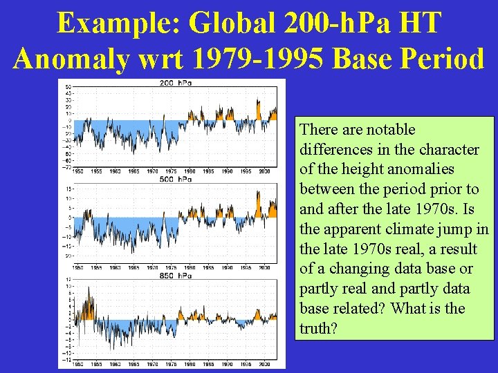
Example: Global 200 -h. Pa HT Anomaly wrt 1979 -1995 Base Period There are notable differences in the character of the height anomalies between the period prior to and after the late 1970 s. Is the apparent climate jump in the late 1970 s real, a result of a changing data base or partly real and partly data base related? What is the truth?

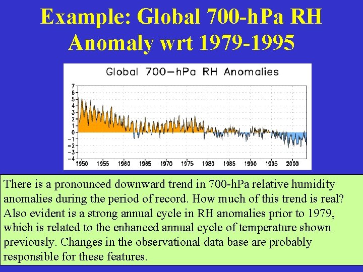
Example: Global 700 -h. Pa RH Anomaly wrt 1979 -1995 There is a pronounced downward trend in 700 -h. Pa relative humidity anomalies during the period of record. How much of this trend is real? Also evident is a strong annual cycle in RH anomalies prior to 1979, which is related to the enhanced annual cycle of temperature shown previously. Changes in the observational data base are probably responsible for these features.

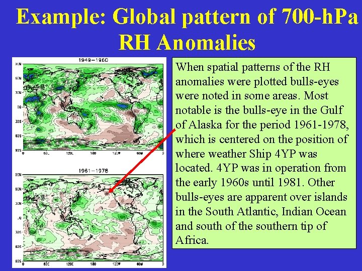
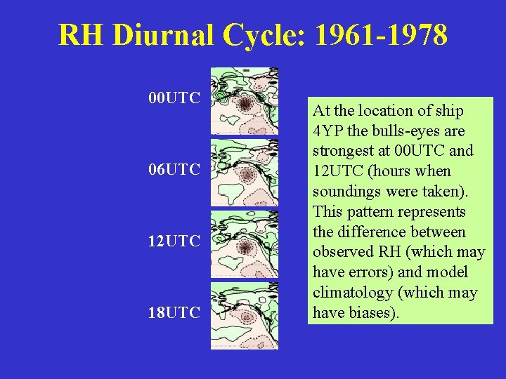
Example: Global pattern of 700 -h. Pa RH Anomalies When spatial patterns of the RH anomalies were plotted bulls-eyes were noted in some areas. Most notable is the bulls-eye in the Gulf of Alaska for the period 1961 -1978, which is centered on the position of where weather Ship 4 YP was located. 4 YP was in operation from the early 1960 s until 1981. Other bulls-eyes are apparent over islands in the South Atlantic, Indian Ocean and south of the southern tip of Africa.

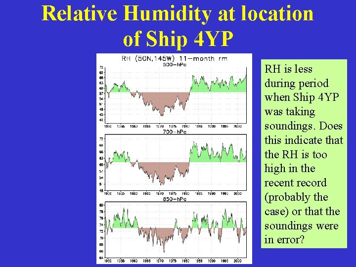
Relative Humidity at location of Ship 4 YP RH is less during period when Ship 4 YP was taking soundings. Does this indicate that the RH is too high in the recent record (probably the case) or that the soundings were in error?

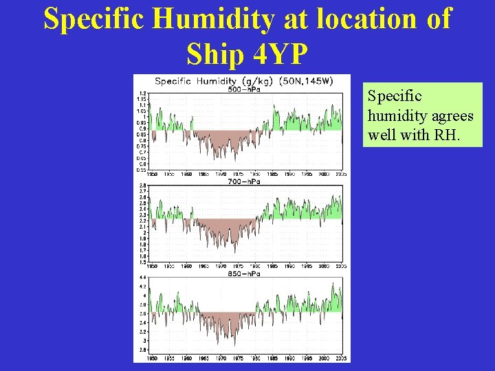
Specific Humidity at location of Ship 4 YP Specific humidity agrees well with RH.

RH Diurnal Cycle: 1961 -1978 00 UTC 06 UTC 12 UTC 18 UTC At the location of ship 4 YP the bulls-eyes are strongest at 00 UTC and 12 UTC (hours when soundings were taken). This pattern represents the difference between observed RH (which may have errors) and model climatology (which may have biases).

Trends: Reality or Fiction? To address this question we • Compare CDAS to AMIP run of GFS (NCEP’s operational global model) - Height and Zonal Wind

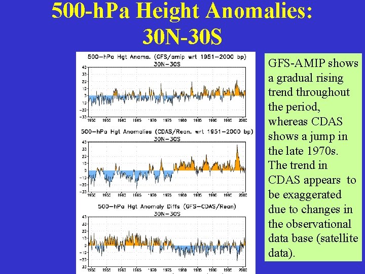
500 -h. Pa Height Anomalies: 30 N-30 S GFS-AMIP shows a gradual rising trend throughout the period, whereas CDAS shows a jump in the late 1970 s. The trend in CDAS appears to be exaggerated due to changes in the observational data base (satellite data).

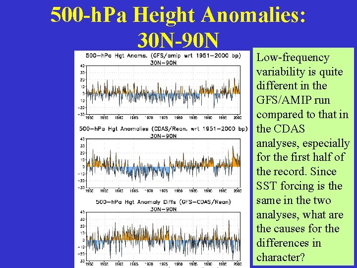
500 -h. Pa Height Anomalies: 30 N-90 N Low-frequency variability is quite different in the GFS/AMIP run compared to that in the CDAS analyses, especially for the first half of the record. Since SST forcing is the same in the two analyses, what are the causes for the differences in character?

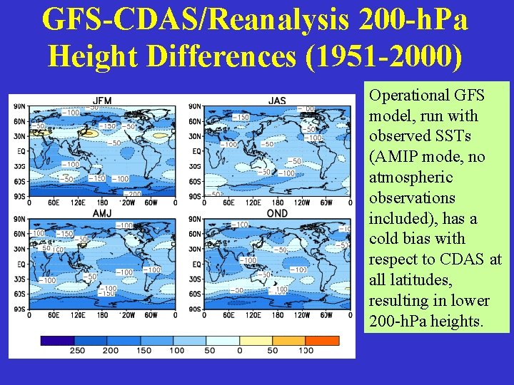
GFS-CDAS/Reanalysis 200 -h. Pa Height Differences (1951 -2000) Operational GFS model, run with observed SSTs (AMIP mode, no atmospheric observations included), has a cold bias with respect to CDAS at all latitudes, resulting in lower 200 -h. Pa heights.

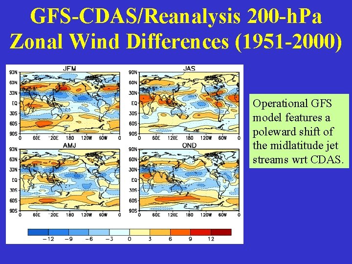
GFS-CDAS/Reanalysis 200 -h. Pa Zonal Wind Differences (1951 -2000) Operational GFS model features a poleward shift of the midlatitude jet streams wrt CDAS.

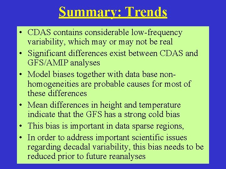
Summary: Trends • CDAS contains considerable low-frequency variability, which may or may not be real • Significant differences exist between CDAS and GFS/AMIP analyses • Model biases together with data base nonhomogeneities are probable causes for most of these differences • Mean differences in height and temperature indicate that the GFS has a strong cold bias • This bias is important in data sparse regions, • In order to address important scientific issues regarding decadal variability, this bias needs to be reduced prior to future reanalyses