Transportation Decision Making Principles of Project Evaluation and

Transportation Decision Making Principles of Project Evaluation and Programming Chapter 18 Evaluation of Transportation Projects and Programs Using Multiple Criteria Kumares C. Sinha and Samuel Labi

n Decision criteria can have multiple dimensions n Dollars n Number of crashes n Acres of land, etc. n All criteria are not of equal importance n For a given criterion, different stakeholders may have different weights.

Typical Steps in Multi-Criteria Decision Making

Establishing Weights n Weights reflect the relative importance attached by decision makers to various criteria n In some cases, the decision maker refers to the agency as well as the facility user. In those cases, the weight used for each criterion is a weighted average of the weights from these two parties.

Weighting Techniques 1. 2. 3. 4. 5. 6. 7. Equal Weights Direct Weighting Derived Weights Delphi Technique Gamble Method Pair-wise comparison: AHP Value Swinging

Equal Weights - Example Project Cost 33. 3% Travel Time Saving 33. 3% VOC Saving 33. 3%

Direct Weighting 1. Point Allocation – A number of points are allocated among the criteria according to their importance. 2. Ranking – Simple ordering by decreasing importance. Point allocation is preferred because unlike ranking, it yields a cardinal rather that an ordinal scale of importance.

Point Allocation (0 -100) (Cardinal) Ranking (Ordinal) Project Cost 70 1 TT Saving 50 3 VOC Saving 60 2

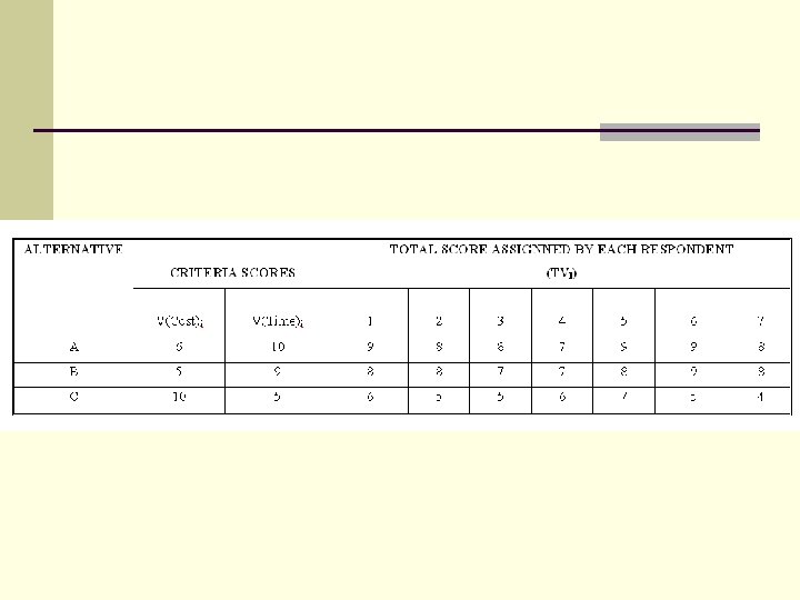
Regression-Based Observer-Derived Weighting 1. Survey respondents assign scores of overall “benefit” or “desirability” for a given combination of criteria levels achieved by each alternative 2. Weights are then the resulting regression coefficients

i = alternative j = Criterion TV = score or desirability

Regression n 7 Respondents n 21 Data Points n TV = wcost* Cost + wtime * Time n n wcost = 0. 214 wtime = 0. 786 R 2 = 0. 98

Delphi Technique n Individual responses aggregated n Effect of assessment of other respondents n Consensus building n Iterative, generally 2 rounds to achieve stable values

Scaling Methods

GAMBLE METHOD 1. Carry out an initial ranking of all criteria in order of decreasing importance. set the first criterion at its most desirable level and all other criteria at their lest desirable levels 2. Compare between the following two outcomes: n n 3. Sure thing: The outcome is that the criterion in question is at its most desirable level while all other criteria at their least desirable levels Gamble: In this outcome, all criteria attained their most desirable levels p% of the time, their least desirable levels (1 -p)% of the time At a certain level of ‘p’ the two situations (sure thing and gamble) are equally desirable. At that level, the value of ‘p’ represents the weight for the criterion in question

Example: Bus Route Assessment Headway (from 5 to 15 minutes) Population Served (from 5, 000 to 10, 000) Solution: 1. Sure Thing: Bus headway is 5 minutes and population served is 5, 000 2. Gamble: Two outcomes: a. A p% chance of an outcome that headway is 5 minutes and population is 10, 000 b. A (1 -p)% chance of an outcome that headway is 15 minutes and population is 5, 000. Suppose the respondent were found to be indifferent between sure thing and gamble at p = 60%, then, the relative weight for bus headway is 0. 6.

Pair Wire Comparison Analytical Hierarchy Process (AHP) = relative importance of two criteria I and j on the basis of a scale of 1 to 9 =

Table 18. 1: Ratios for Pair wise Comparison Matrix

Value Swinging Method 1. 2. 3. 4. Consider a hypothetical situation where all criteria at their worst values Determine the criterion for which it is most preferred to “swing” from its worst value to best value, all other criteria remaining at their worst values. Repeat steps 1 and 2 for all criteria. Assign the most important criterion the highest weight in a selected weighting range (100 for 1 -100 scale) and then assign weights to the remaining criteria in proportion to their rank of importance.

Scaling of Performance Criteria Certainty - Value Function Risk - Utility Function Uncertainty - Scenario Analysis

Value Function a. Direct Rating Method – direct assignment of value to various levels of a criterion b. Mid Value Splitting Technique – based on “indifference” between changes in levels of criterion. c. Regression – based on data from direct rating

Discrete Value Function

Continuous Value Function

Developed Value Functions

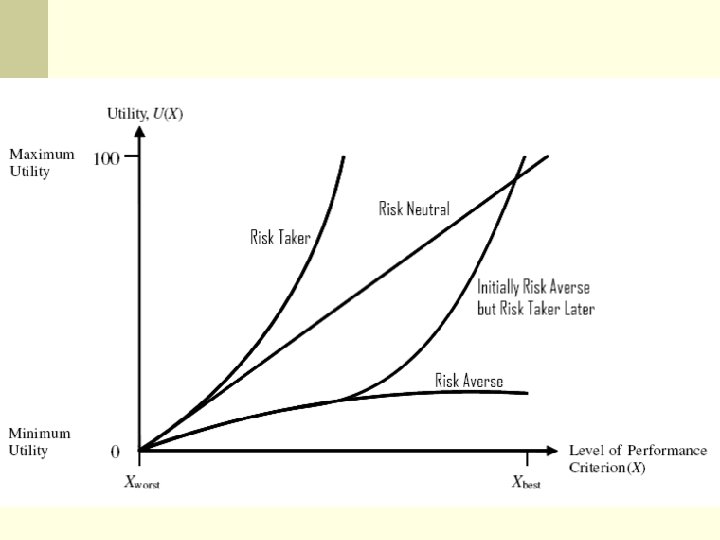
Utility Function Direct Questioning Using the Gamble Approach Guaranteed prospect of an outcome vs. risky prospect of a more favorable outcome.

Example 18. 7 n Utility Functions for agency cost, ecological damage, and vulnerable population served. Solution: For Agency Cost: Ucost ($30 Million) = 0 (Worst) Ucost ($ 0 Million) = 1 (Best) Sure Thing: The outcome is that agency cost is guaranteed to be $20 Million Gamble: There is a 50% chance that cost is 0 and 50% change it is $30 Million X 50 = $20 Million is the Certainty Equivalent because the expected utility is 0. 5

Cost (in $millions) Population served (in thousands) Wetland lost in acres (in tens)

Combination of Performance Criteria n Pareto Optimality n Difference Approach n Net Utility = U(B) – U(C) n NPV = PV (B) – PV(C) n Ratio Approach n Utility Ratio = U(B)/U(C) n BCR = PV(B) / PV(C)

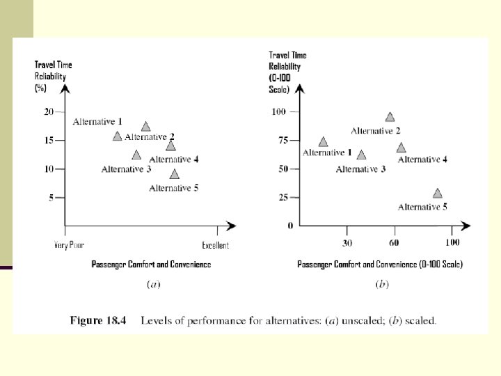
Cost Effectiveness n Costs and Benefits are not necessarily expressed in the same metrics n Indifference Curves n Tradeoffs – marginal rates of substitution between criteria n TV = 2*TTR + PCC

Indifference Curves Using Mathematical Form of Utility/Value Function for Combined Performance Measures

Ranking and Rating Method

Impact Index Method

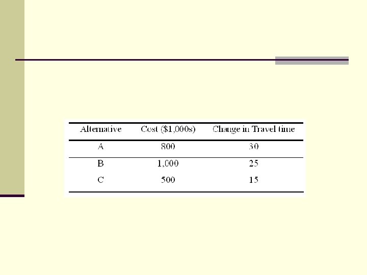
Table E 18. 10. 1: Performance of Alternatives

Figure E 18. 10: Plot of Confidence Intervals