Transformations to Achieve Linearity Common Models for Curved

Transformations to Achieve Linearity

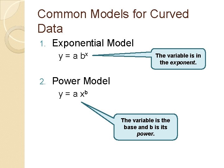
Common Models for Curved Data 1. Exponential Model y = a bx 2. The variable is in the exponent. Power Model y = a xb The variable is the base and b is its power.

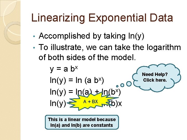
Linearizing Exponential Data Accomplished by taking ln(y) • To illustrate, we can take the logarithm of both sides of the model. y = a bx Need Help? Click here. ln(y) = ln (a bx) ln(y) = ln(a) + ln(bx) A + BX ln(y) = ln(a) + ln(b)x • This is a linear model because ln(a) and ln(b) are constants

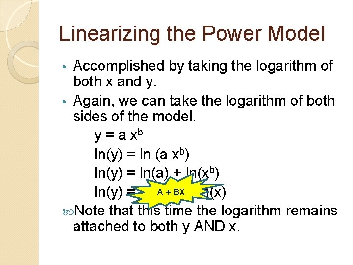
Linearizing the Power Model Accomplished by taking the logarithm of both x and y. • Again, we can take the logarithm of both sides of the model. y = a xb ln(y) = ln (a xb) ln(y) = ln(a) + ln(xb) A++ BX b ln(x) ln(y) = ln(a) Note that this time the logarithm remains attached to both y AND x. •

Why Should We Linearize Data? Much of bivariate data analysis is built on linear models. By linearizing nonlinear data, we can assess the fit of non-linear models using linear tactics. In other words, we don’t have to invent new procedures for non-linear data. HOORAY!!

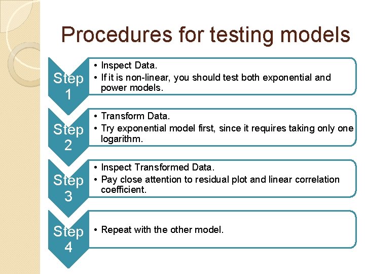
Procedures for testing models Step 1 Step 2 Step 3 Step 4 • Inspect Data. • If it is non-linear, you should test both exponential and power models. • Transform Data. • Try exponential model first, since it requires taking only one logarithm. • Inspect Transformed Data. • Pay close attention to residual plot and linear correlation coefficient. • Repeat with the other model.

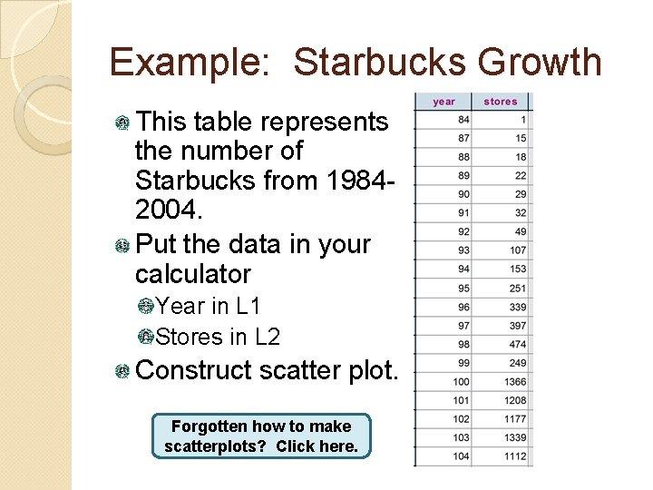
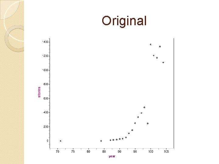
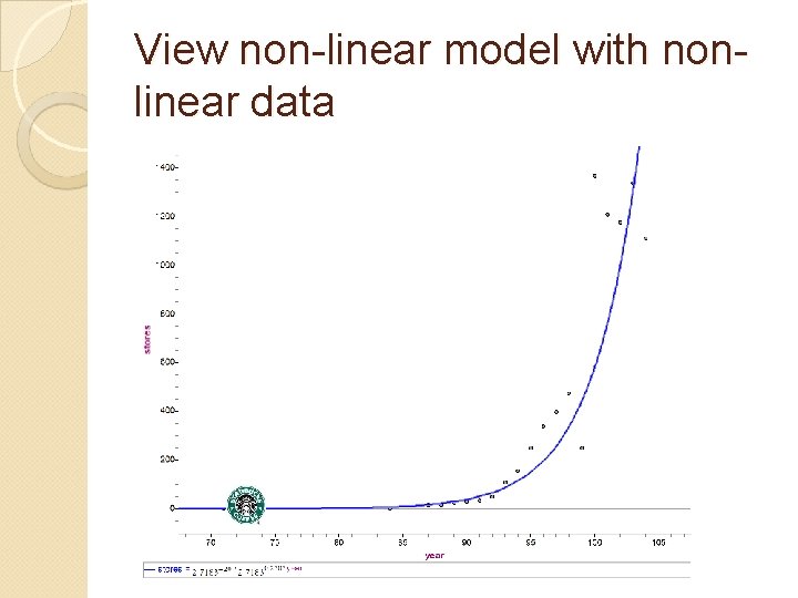
Example: Starbucks Growth This table represents the number of Starbucks from 19842004. Put the data in your calculator Year in L 1 Stores in L 2 Construct scatter plot. Forgotten how to make scatterplots? Click here.

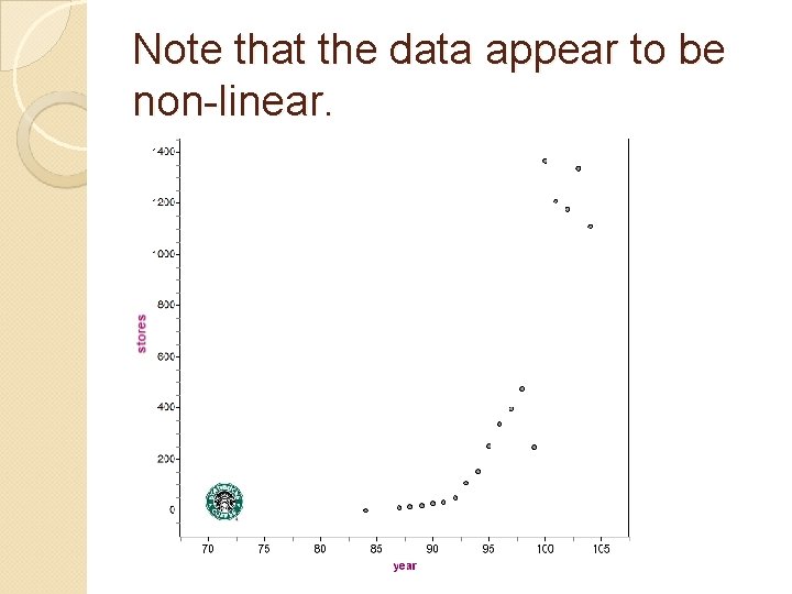
Note that the data appear to be non-linear.

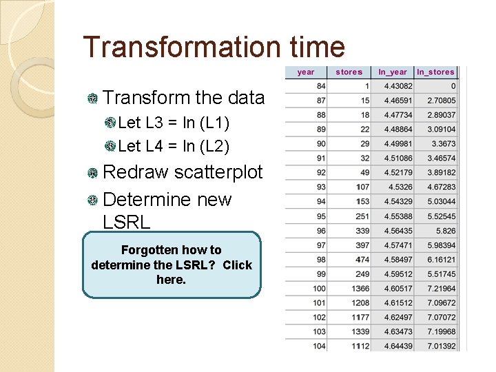
Transformation time Transform the data Let L 3 = ln (L 1) Let L 4 = ln (L 2) Redraw scatterplot Determine new LSRL Forgotten how to determine the LSRL? Click here.

Original

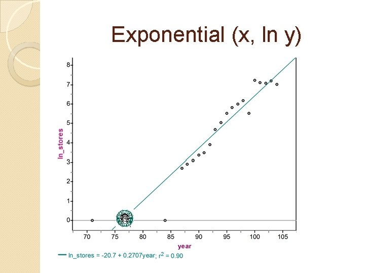
Exponential (x, ln y)

Original

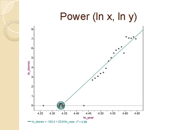
Power (ln x, ln y)

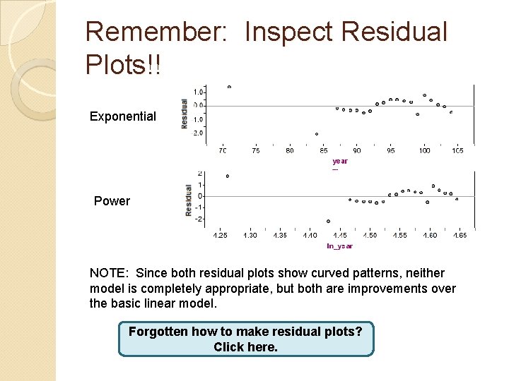
Remember: Inspect Residual Plots!! Exponential Power NOTE: Since both residual plots show curved patterns, neither model is completely appropriate, but both are improvements over the basic linear model. Forgotten how to make residual plots? Click here.

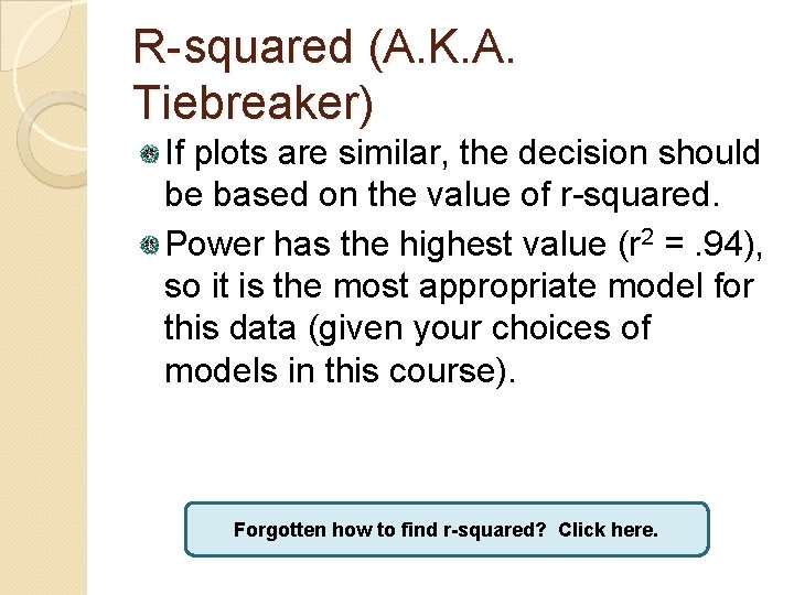
R-squared (A. K. A. Tiebreaker) If plots are similar, the decision should be based on the value of r-squared. Power has the highest value (r 2 =. 94), so it is the most appropriate model for this data (given your choices of models in this course). Forgotten how to find r-squared? Click here.

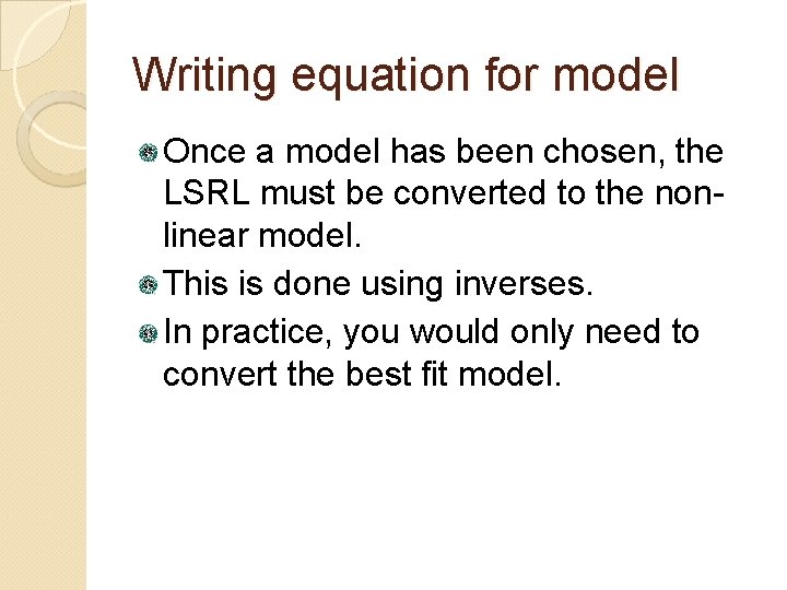
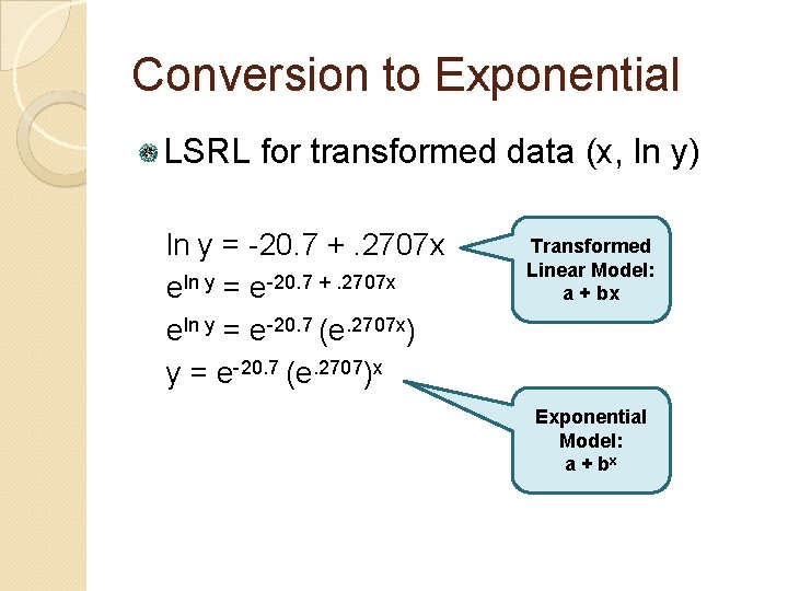
Writing equation for model Once a model has been chosen, the LSRL must be converted to the nonlinear model. This is done using inverses. In practice, you would only need to convert the best fit model.

Conversion to Exponential LSRL for transformed data (x, ln y) ln y = -20. 7 +. 2707 x eln y = e-20. 7 (e. 2707 x) y = e-20. 7 (e. 2707)x Transformed Linear Model: a + bx Exponential Model: a + bx

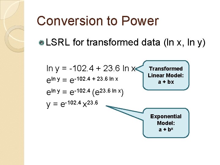
Conversion to Power LSRL for transformed data (ln x, ln y) ln y = -102. 4 + 23. 6 ln x eln y = e-102. 4 (e 23. 6 ln x) y = e-102. 4 x 23. 6 Transformed Linear Model: a + bx Exponential Model: a + bx

View non-linear model with nonlinear data