Transformations Transformations to Linearity Many nonlinear curves can

Transformations

Transformations to Linearity • Many non-linear curves can be put into a linear form by appropriate transformations of the either – the dependent variable Y or – some (or all) of the independent variables X 1, X 2, . . . , Xp. • This leads to the wide utility of the Linear model. • We have seen that through the use of dummy variables, categorical independent variables can be incorporated into a Linear Model. • We will now see that through the technique of variable transformation that many examples of non -linear behaviour can also be converted to linear behaviour.

Intrinsically Linear (Linearizable) Curves 1 Hyperbolas y = x/(ax-b) Linear form: 1/y = a -b (1/x) or Y = b 0 + b 1 X Transformations: Y = 1/y, X=1/x, b 0 = a, b 1 = -b

2. Exponential y = a ebx = a. Bx Linear form: ln y = lna + b x = lna + ln. B x or Y = b 0 + b 1 X Transformations: Y = ln y, X = x, b 0 = lna, b 1 = b = ln. B

3. Power Functions y = a xb Linear from: ln y = lna + blnx or Y = b 0 + b 1 X

Logarithmic Functions y = a + b lnx Linear from: y = a + b lnx or Y = b 0 + b 1 X Transformations: Y = y, X = ln x, b 0 = a, b 1 = b

Other special functions y = a e b/x Linear from: ln y = lna + b 1/x or Y = b 0 + b 1 X Transformations: Y = ln y, X = 1/x, b 0 = lna, b 1 = b

Polynomial Models y = b 0 + b 1 x + b 2 x 2 + b 3 x 3 Linear form Y = b 0 + b 1 X 1 + b 2 X 2 + b 3 X 3 Variables Y = y, X 1 = x , X 2 = x 2, X 3 = x 3

Exponential Models with a polynomial exponent Linear form lny = b 0 + b 1 X 1 + b 2 X 2 + b 3 X 3+ b 4 X 4 Y = lny, X 1 = x , X 2 = x 2, X 3 = x 3, X 4 = x 4

Trigonometric Polynomial Models y = b 0 + g 1 cos(2 pf 1 x) + d 1 sin(2 pf 1 x) + … + gkcos(2 pfkx) + dksin(2 pfkx) Linear form Y = b 0 + g 1 C 1 + d 1 S 1 + … + gk Ck + dk Sk Variables Y = y, C 1 = cos(2 pf 1 x) , S 2 = sin(2 pf 1 x) , … Ck = cos(2 pfkx) , Sk = sin(2 pfkx)

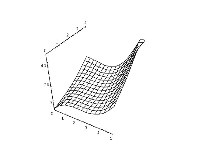
Response Surface models Dependent variable Y and two independent variables x 1 and x 2. (These ideas are easily extended to more the two independent variables) The Model (A cubic response surface model) or Y = b 0 + b 1 X 1 + b 2 X 2 + b 3 X 3 + b 4 X 4 + b 5 X 5 + b 6 X 6 + b 7 X 7 + b 8 X 8 + b 9 X 9+ e where

The Box-Cox Family of Transformations

The Transformation Staircase

The Bulging Rule y up x down x up y down

Non-Linear Models Nonlinearizable models

Non-Linear Growth models • many models cannot be transformed into a linear model The Mechanistic Growth Model Equation: or (ignoring e) “rate of increase in Y” =

The Logistic Growth Model Equation: or (ignoring e) “rate of increase in Y” =

The Gompertz Growth Model: Equation: or (ignoring e) “rate of increase in Y” =

Example: daily auto accidents in Saskatchewan to 1984 to 1992 Data collected: 1. Date 2. Number of Accidents Factors we want to consider: 1. Trend 2. Yearly Cyclical Effect 3. Day of the week effect 4. Holiday effects

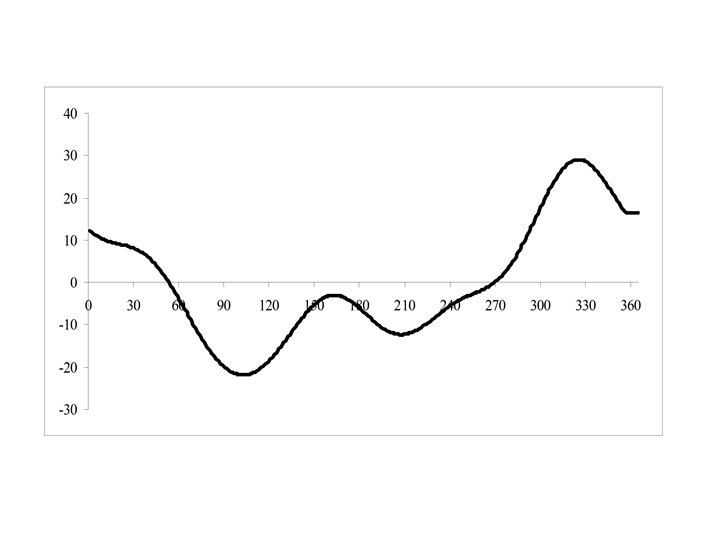
Trend This will be modeled by a Linear function : Y = b 0 +b 1 X (more generally a polynomial) Y = b 0 +b 1 X +b 2 X 2 + b 3 X 3 + …. Yearly Cyclical Trend This will be modeled by a Trig Polynomial – Sin and Cos functions with differing frequencies(periods) : Y = d 1 sin(2 pf 1 X) + g 1 cos(2 pf 2 X) + d 1 sin(2 pf 2 X) + g 2 cos(2 pf 2 X) + …

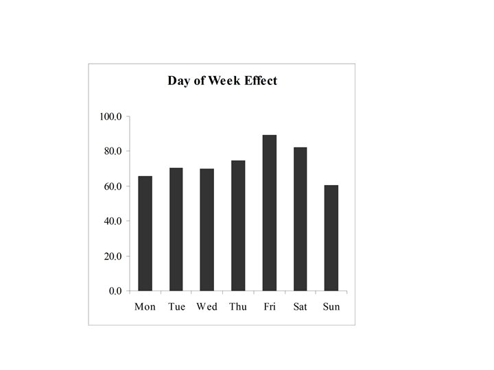
Day of the week effect: This will be modeled using “dummy”variables : a 1 D 1 + a 2 D 2 + a 3 D 3 + a 4 D 4 + a 5 D 5 + a 6 Di = (1 if day of week = i, 0 otherwise) Holiday Effects Also will be modeled using “dummy”variables :

Independent variables X = day, D 1, D 2, D 3, D 4, D 5, D 6, S 1, S 2, S 3, S 4, S 5, S 6, C 1, C 2, C 3, C 4, C 5, C 6, NYE, HW, V 1, V 2, cd, T 1, T 2. Si=sin(0. 017202423838959*i*day). Ci=cos(0. 017202423838959*i*day). Dependent variable Y = daily accident frequency

Independent variables ANALYSIS OF VARIANCE SUM OF SQUARES DF MEAN SQUARE F RATIO REGRESSION 976292. 38 18 54238. 46 114. 60 RESIDUAL 1547102. 1 3269 473. 2646 VARIABLES IN EQUATION FOR PACC VARIABLES NOT IN EQUATION STD. ERROR STD REG F . PARTIAL F VARIABLE COEFFICIENT OF COEFF TOLERANCE TO REMOVE LEVEL. VARIABLE CORR. TOLERANCE TO ENTER LEVEL (Y-INTERCEPT 60. 48909 ) . day 1 0. 11107 E-02 0. 4017 E-03 0. 038 0. 99005 7. 64 1. IACC 7 0. 49837 0. 78647 1079. 91 0 D 1 9 4. 99945 1. 4272 0. 063 0. 57785 12. 27 1. Dths 8 0. 04788 0. 93491 7. 51 0 D 2 10 9. 86107 1. 4200 0. 124 0. 58367 48. 22 1. S 3 17 -0. 02761 0. 99511 2. 49 1 D 3 11 9. 43565 1. 4195 0. 119 0. 58311 44. 19 1. S 5 19 -0. 01625 0. 99348 0. 86 1 D 4 12 13. 84377 1. 4195 0. 175 0. 58304 95. 11 1. S 6 20 -0. 00489 0. 99539 0. 08 1 D 5 13 28. 69194 1. 4185 0. 363 0. 58284 409. 11 1. C 6 26 -0. 02856 0. 98788 2. 67 1 D 6 14 21. 63193 1. 4202 0. 273 0. 58352 232. 00 1. V 1 29 -0. 01331 0. 96168 0. 58 1 S 1 15 -7. 89293 0. 5413 -0. 201 0. 98285 212. 65 1. V 2 30 -0. 02555 0. 96088 2. 13 1 S 2 16 -3. 41996 0. 5385 -0. 087 0. 99306 40. 34 1. cd 31 0. 00555 0. 97172 0. 10 1 S 4 18 -3. 56763 0. 5386 -0. 091 0. 99276 43. 88 1. T 1 32 0. 00000 0. 00 1 C 1 21 15. 40978 0. 5384 0. 393 0. 99279 819. 12 1. C 2 22 7. 53336 0. 5397 0. 192 0. 98816 194. 85 1. C 3 23 -3. 67034 0. 5399 -0. 094 0. 98722 46. 21 1. C 4 24 -1. 40299 0. 5392 -0. 036 0. 98999 6. 77 1. C 5 25 -1. 36866 0. 5393 -0. 035 0. 98955 6. 44 1. NYE 27 32. 46759 7. 3664 0. 061 0. 97171 19. 43 1. HW 28 35. 95494 7. 3516 0. 068 0. 97565 23. 92 1. T 2 33 -18. 38942 7. 4039 -0. 035 0. 96191 6. 17 1. ***** F LEVELS( 4. 000, 3. 900) OR TOLERANCE INSUFFICIENT FOR FURTHER STEPPING

Day of the week effects D 1 4. 99945 D 2 9. 86107 D 3 9. 43565 D 4 13. 84377 D 5 28. 69194 D 6 21. 63193

Holiday Effects NYE HW T 2 32. 46759 35. 95494 -18. 38942

Cyclical Effects S 1 S 2 S 4 C 1 C 2 C 3 C 4 C 5 -7. 89293 -3. 41996 -3. 56763 15. 40978 7. 53336 -3. 67034 -1. 40299 -1. 36866

Transformations to Linearity • Many non-linear curves can be put into a linear form by appropriate transformations of the either – the dependent variable Y or – some (or all) of the independent variables X 1, X 2, . . . , Xp. • This leads to the wide utility of the Linear model. • We have seen that through the use of dummy variables, categorical independent variables can be incorporated into a Linear Model. • We will now see that through the technique of variable transformation that many examples of non -linear behaviour can also be converted to linear behaviour.

Intrinsically Linear (Linearizable) Curves 1 Hyperbolas y = x/(ax-b) Linear form: 1/y = a -b (1/x) or Y = b 0 + b 1 X Transformations: Y = 1/y, X=1/x, b 0 = a, b 1 = -b

2. Exponential y = a ebx = a. Bx Linear form: ln y = lna + b x = lna + ln. B x or Y = b 0 + b 1 X Transformations: Y = ln y, X = x, b 0 = lna, b 1 = b = ln. B

3. Power Functions y = a xb Linear from: ln y = lna + blnx or Y = b 0 + b 1 X

Logarithmic Functions y = a + b lnx Linear from: y = a + b lnx or Y = b 0 + b 1 X Transformations: Y = y, X = ln x, b 0 = a, b 1 = b

Other special functions y = a e b/x Linear from: ln y = lna + b 1/x or Y = b 0 + b 1 X Transformations: Y = ln y, X = 1/x, b 0 = lna, b 1 = b

Polynomial Models y = b 0 + b 1 x + b 2 x 2 + b 3 x 3 Linear form Y = b 0 + b 1 X 1 + b 2 X 2 + b 3 X 3 Variables Y = y, X 1 = x , X 2 = x 2, X 3 = x 3

Exponential Models with a polynomial exponent Linear form lny = b 0 + b 1 X 1 + b 2 X 2 + b 3 X 3+ b 4 X 4 Y = lny, X 1 = x , X 2 = x 2, X 3 = x 3, X 4 = x 4

Trigonometric Polynomials

• b 0, d 1, g 1, … , dk, gk are parameters that have to be estimated, • n 1, n 2, n 3, … , nk are known constants (the frequencies in the trig polynomial. Note:

Response Surface models Dependent variable Y and two independent variables x 1 and x 2. (These ideas are easily extended to more the two independent variables) The Model (A cubic response surface model) or Y = b 0 + b 1 X 1 + b 2 X 2 + b 3 X 3 + b 4 X 4 + b 5 X 5 + b 6 X 6 + b 7 X 7 + b 8 X 8 + b 9 X 9+ e where

The Box-Cox Family of Transformations

The Transformation Staircase

The Bulging Rule y up x down x up y down